Both Trak and OmniTrak can include contibutions of cathode temperature to the emittance of extracted electron beams. The theory of how the thermal energy of electrons emitted a hot cathode appears as an angular beam divergence is discussed in Sect. 10.3 of the Trak manual and Sect. 11.2 of the OmniTrak manual.
Using the thermal feature involves some setup effort and decisions, so that new users may not be confident of their results. In this article, I review setup procedures for both Trak and OmniTrak runs. Most important, I'll show the codes agree with each other and that the results are physically reasonable. Code users can download the input files using the link at the end of the article.
We'll start with the Trak calculation of the electron gun (run prefix HOTCATHODETRAK). Figure 1 shows the geometry. The cathode, focus electrode and emission surface were at -10.0 kV and the anode was at ground potential. The calculation was performed in the SCharge mode. The emission surface that covered the planar cathode had region number RegNo = 3. Space-charge limited emission for a cold cathode is controlled by the following command in the Trak input script HOTCATHODETRAK.TIN:
EMIT(3): 0.0000E+00 -1.0000E+00 5.0000E-02 2
This form of the command applies to a cold cathode. The first two parameters (0.0 and -1.0) signal that the emitted particles are electrons. The third parameter is the distance from the physical cathode surface to the virtual emission surface, 0.05 cm (two element widths). At this spacing, the potential at the virtual emission surface was about 50-100 V. The final parameter is the number of model electrons to create per facet of the emission surface.
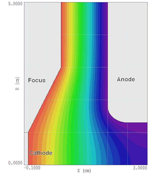
Figure 1. Gun geometry of the Trak simulation, a z-r plot for the cylindrically-symmetric system.
The cold-cathode calculation gave the model electron trajectories shown in Fig. 2. The initially-parallel beam diverged because of the negative lens effect at the extraction aperture. The space-charge-limited current was 1.432 A.
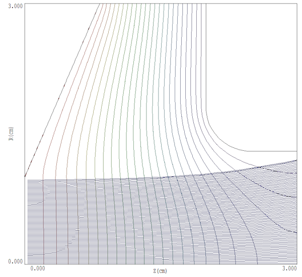
Figure 2. Self-consistent model electron trajectories, Trak calculation.
The top illustration of Fig. 3 (created with GenDist) shows the radial phase-space distribution of the exit beam. It follows a line of effectively zero thickness. The line is not straight because focusing forces in the gun do not vary linearly with r.
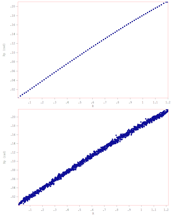
Figure 3. Phase space distribution of the exit beam, Trak calculation. Top: Cold cathode. Bottom: Cathode temperature kT/e = 0.2 eV.
To model a hot cathode, the emission command was modified to
EMIT(3): 0.0000E+00 -1.0000E+00 5.0000E-02 2 1.0E4 0.2 20
There are three extra parameters. The number 1.0E4 was a source limit on current density. In this case, the number was acting only as a placeholder and was set to a value much higher than the expected space-charge limit. The number 0.2 was the cathode temperature in eV. In order to calculate initial angles, it is important that this number be small compared to the electrostatic potential of the virtual emission surface. Finally, the number of 20 is a statistical splitting factor. Each model particle was split into 20 independently-emitted sub-particles for a total of 1369 to give an accurate phase-space distribution. The bottom illustration in Fig. 3 shows the results. The phase-space distribution r-rp shows the spread in radial angle. Measuring the graph with the Universal Scale, I found that the angular spread was about 0.005 radians. For comparison, the predicted angular spread is on the order of (kT/Te), where Te is the exit energy in eV. Taking kT = 0.2 and Te = 1.0E4, the value is about 0.0045 radians.
I modeled the same geometry with OmniTrak (run prefix HOTCATHODEOMNITRAK). To minimize the run time, the solution volume include only the first quadrant, with field symmetry and particle reflection boundaries at x = 0.0 cm and y = 0.0 cm. The MetaMesh input file (HOTCATHODEOMNITRAK.MIN) demonstrates the construction of an accurate emission surface (Fig.4). The emission commands in the OmniTrak input file HOTCATHODEOMNITRAK.OIN had the form:
EMIT(4): 0.0000E+00 -1.0000E+00 3.0000E-02 2
TSOURCE 0.2
The parameter 2 in the EMIT command signifies that 2^2 particles are emitted from each facet of the emission surface, for a total of 5024. The calculation gave a space-charge-limited current of 0.364248 A/quadrant. The total current of 1.456 A was within 1.4% of the Trak prediction. Figure 5 shows the resulting radial phase-space distribution. The top illustration is for a cold beam with the TSOURCE command commented out. The bottom illustration shows the warm beam results. The exit beam was slightly larger than the Trak prediction and there is a little structure on the envelope. The behavior of particles on the envelope was highly sensitive to interpolations of the edge field, and there were small errors in the 3D calculation. The warm beam result was almost identical to the Trak calculation.
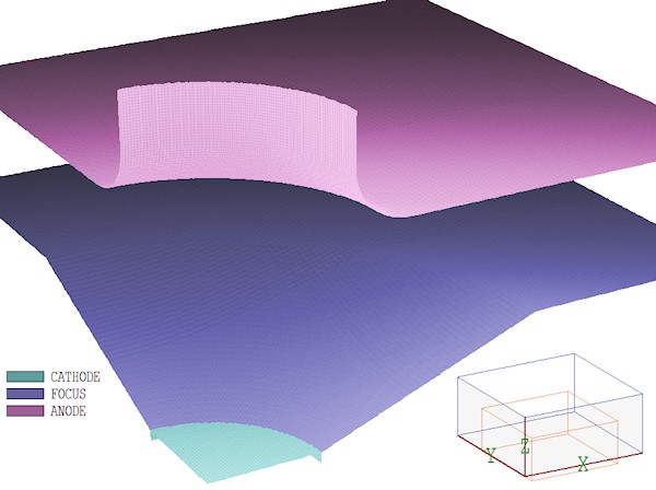
Figure 4. Surfaces for the OmniTrak calculation as represented by MetaMesh.
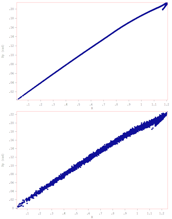
Figure 5. Phase space distribution of the exit beam, OmniTrak calculation. Top: Cold cathode. Bottom: Cathode temperature kT/e = 0.2 eV.
Trak and OmniTrak users, link to download input files: HotCathodeDemo.zip
LINKS
