PerMag and Magnum calculate magnetostatic fields in 2D and 3D geometries. An noteworthy feature of the programs is the ability to represent saturation effects in iron-like materials (i.e., non-linear solutions). To perform the calculations, the programs require data on the response of the specific materials. The two programs use different calculation methods, so they require different data forms:
- PerMag expects a table of values of B-μr, where B is the magnetic flux density inside the material and μr is the relative magnetic permeability.
- Magnum expects a table of B0-μr, where B0 = μ0*H (the applied magnetic field).
We supply tables for a broad range of materials with the software packages. A useful feature of both programs is that you can create your own tables to represent any magnetic materials.
The purpose of this article is to step through the creation of tables for some challenging materials, showing strategies for good data representations. I created new tables for two types of MetGlas materials as part of a consulting job and added them to the PerMag and Magnum material libraries.
Figure 1 shows the type of raw data you may encounter. It was taken from a pdf techsheet document from MetGlas Inc. for Hitachi material 2605HB1M. The quoted saturation magnetic flux is Bs = 1.63 T. The graph is a static hysteresis curve showing B versus H. We shall use the blue curve that extends to the highest values of H. Some hysteresis is apparent — the curve follows a different trajectory on the way down (left-hand-side) than the way up. The small difference is not important in static calculations, so I chose to digitize the right-hand curve and shift it so that it passed through the origin.
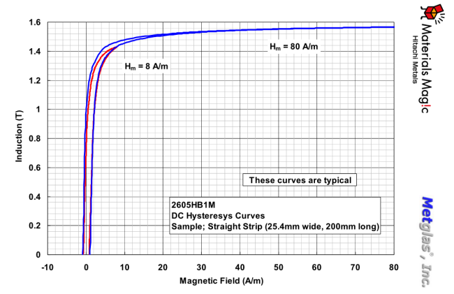
Figure 1. Example of available data, MetGlas 2605HB1M.
This was good opportunity to use our freeware utility FPUniscale to determine a set of values for B-H directly from a screen display of Fig. 1. Figure 2 shows the setup for using FPUniscale The setup for onscreen digitizing in the picture shows a later stage of this calculation, so I'll delay discussing the details. For now, accept that I used FPUniscale to generate a comma-delimited file of 25 values of B-H over the range of the H axis.
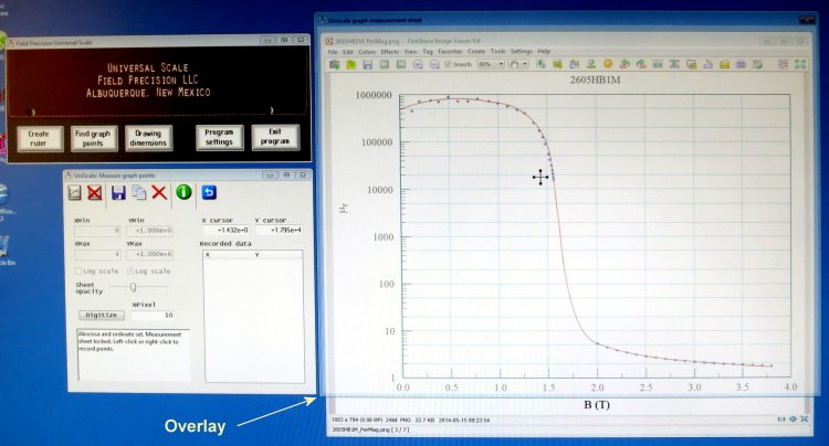
Figure 2. Operation of FPUniscale.
The values can be transferred directly to a spreadsheet as shown in Fig. 3 (columns 1 and 2). The measured values are above the red arrow. In Column3, the H values are shifted to pass through the origin and scaled to represent the applied flux density B0 = μ0*H. The relative permeability in column 4 is simply B/B0.
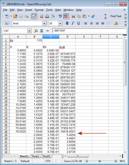
Figure 3. Spreadsheet to find the relative permeability.
As they stand, the values given in Fig. 1 are of no use for modeling saturation effects. The range of applied magnetic flux density is quite small (B0 ≪ Bs) and the values of relative magnetic permeability are consistently high (μr ≫ 1). As discussed in other articles, there is no need to use a permeability table for calculations in this range. A linear material with a high fixed value of μr would give almost identical results. For saturation modeling, we need to extend the curve to high values of B0 where μr approaches 1.0. This is where some insights and strategies are required.
As discussed in a previous article, we can approximate the relative permeability of all non-linear materials in the region B > Bs with the formula
?r?? B/(B - Bs),
where Bs is the saturation flux density. The values below the red arrow in Fig. 3 were calculated from the equation. I copied and pasted the full set of values into Psi-Plot. After some experimentation with axis types, I created the graph shown in Fig. 4 (appropriate for PerMag). The two groups of values are shown as blue circles. The compelling aspect of the plot is that even though the groups are widely separated, it is clear how they must connect. Accordingly, I ported the graph to Paintshop Pro and worked with Bezier curves to create the red line in Fig. 4. There is of course some guesswork, but the actual values can't be too far from the estimate shown. The interpolation is more self-evident in a plot of B0-?r values for Magnum (Fig. 5). Because of the wide range of B0 values, I used log intervals along both axis. In this case, the interpolation is close to a straight line.

CAPTION
[caption id="" align="aligncenter" width="700"]

Figure 4. Interpolated curve (material 2605HB1M) for PerMag.[/caption]
CAPTION
[caption id="" align="aligncenter" width="700"]

Figure 5. Interpolated curve (material 2605HB1M) for Magnum.[/caption]
The final step is to digitize the curves of Figs. 4 and 5 using FPUniscale. In preparation, I displayed the graph in FastStone Image Viewer. With reference to Fig. 2, I ran FPUniscale and picked the option Find graph points from the main window (top-left). A setup window (bottom-left) appears. I entered the values 0 and 4 for the limits of the x axis. I set the y axis as log and entered the limits 1 and 1000000. I then clicked the Open measurements sheet tool to create a transparent overlay (yellow arrow). After moving and resizing it to overlap the graph, I set the origin and the two maximum points on the axes. Calibration of the digitizer is shown as blue lines in Fig. 2. Then it remained to move the cursor to several points along the graph, clicking the mouse to add values to the list box in the setup window. When complete, I clicked the Save data to file tool to create a comma-delimited text file. The data were added as files to the PerMag and Magnum libraries and added to our tech sheet of saturation curves.
This was a satisfying project for two reasons:
- I got to use many of my favorite programs.
- It demonstrated the power of human pattern recognition. It is obvious to a person how to draw the connecting curves in Figs. 4 and 5, but I suspect it would have taken hours of work fiddling with fitting functions on a computer to attain the same result.
Figure 6 shows a test of the model in a PerMag solution, a simple geometry with a MetGlas core enclosing a drive coil. In the top picture, the applied field is low (B0?? Bs), so the core acts like an ideal pole (lines of B enter normal to the surface). The coil current is high in the bottom picture, producing regions of saturation inside the core leading to an interesting field pattern. Because of the strong non-linearity of the B-?r curves, it was necessary to use a low value of material adjustment parameter (Avg = 0.02) and a large number of cycles (N = 10,000) to achieve a stable, well-converged solution.
[caption id="" align="aligncenter" width="550"]

Figure 6. PerMag solutions with material 2605HB1M. Top: no saturation. Bottom: high saturation.[/caption]
Footnotes
[1] Contact us :?techinfo@fieldp.com.
[2] Field Precision home page: www.fieldp.com.
LINKS
