In finite-element solutions at low magnetic fields, the properties of ferromagnetic materials are not critically important. The quantity used in the solutions is γ = 1/μr. In this case, both 1/800 and 1/8000 are close to zero compared to unity; therefore, the details of the μr(B) curve make little difference in the solution. On the other hand, the variation of relative permeability may be quite important at high field levels where the materials are driven into saturation. Unfortunately, the available data in tabulations of μr(B) are generally the inverse of what we need: there is extensive information at low B but most tabulations end well below the saturation region. The subject of this article is how to guess μr(B) at high field levels from the low-field behavior. Sounds impossible, but its actually easy thanks to two factors:
- Magnetic saturation occurs smoothly (i.e., there are no abrupt changes).
- We know the variation at extremely high fields.
The key is choosing a good method to plot the data.
First, some background. The typical measurement setup is a torus of material with a drive coil winding. The quantity H (in A/m) is the magnetic field produced by the coil in the absence of the material. A useful quantity is B0 = μ0*H (in Tesla), the magnetic flux density produced by the coil inside the torus with no material. The quantity B is the total flux density in the torus with the material present. In this case, alignment of atomic currents adds to the field value so that B > B0. In a soft magnetic material (i.e., no permanent magnetization), both B0 and B equal zero when there is no drive current. The alignment of magnetic domains increases as the drive current increases; therefore, B grows faster than B0. The relative magnetic permeability is defined as μr = B/B0. At high values of drive current, all the material domains have been aligned. In this state, the material makes a maximum contribution to the total flux density of Bs (the saturation flux density). This contribution does not change with higher drive current. For high values of B0, the total flux density is approximated by
B ≅ B0 + Bs. (1)
To illustrate the estimation procedure, we'll consider the specific example of Magnifer 50 RG, a nickle alloy with a high value of Bs. Figure 1 shows a graph from a data sheet supplied by VDM Metals. The sheet lists the saturation flux density as Bs = 1.55 T. The plot shows B (in mT) versus H (mA/cm) at several frequencies. Because we are interested in the static properties, we'll consider only curve 1. The data extend to a peak value of H = 200 A/m. At this point, µr? 1000, so that the material is well below saturation. I have an application where the material is driven well into to saturation by applied fields up to H = 5000 A/m, about 400 times the highest known value! Is it possible to make calculations with confidence?
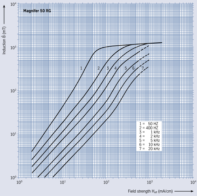
Figure 1. Data from VDM Metals on Magnifer 50 RG, B versus H.
The first step is convert the graphics data to a number set. The FP Universal Scale is the ideal tool for this task. After setting the correct log scales, I could record a set of points with simple mouse clicks, including the conversion factors to create a list of B versus B0 in units of Tesla. In this case, the relative magnetic permeability is the ratio µr = B/B0.
The key to estimating the missing values is to create plots of the material behavior at the two extremes: the tabulated values at low B0 and predictions from Eq. 1 at high B0. To ensure the validity of Eq. 1, I picked B0 values corresponding to highly saturated material: 0.1, 0.2 and 0.5 T. The art is picking the right type of plot. Figure 2 shows B versus B0 with log-log scales. With the requirement of a smooth variation, clearly the unknown values must lie close to the dashed red line connecting the data extremes. Accordingly, I used the Universal Scale to find several points along the line. I combined the interpolated values with the low field tabulated values and the high-field predictions to build a data set that spans the complete range of behavior for Magnifer 50.
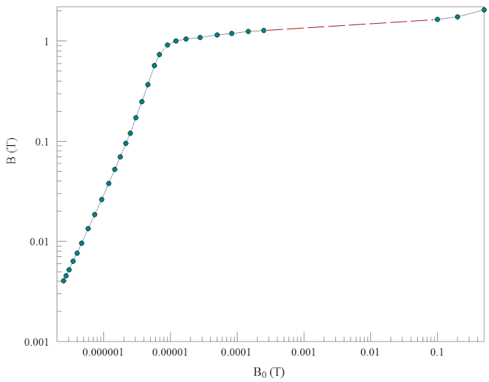
Figure 2. Plot of B versus B0 for Magnifer 50 showing values at high and low field with a proposed interpolation (dashed red line).
Finally, Figure 3 shows alternate plots to Fig. 2: B0 versus μr and B versus μr. In all cases, the variation over the unknown saturation region is well approximated by a simple straight-line fit.
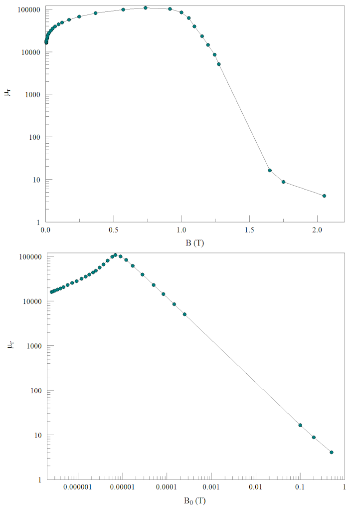
Figure 3. Alternative plots and interpolations for Magnifer 50 RG: B0 and B versus relative magnetic permeability.
LINKS
