|
Input files
|
Loop3D.CDF, Loop3D.MIN, Loop3D.GIN, Loop3D.SCR
LoopInduct3D.zip
|
|
Description
|
The example is the third in a series illustrating techniques for self and mutual inductance calculations with PerMag, Nelson and Magnum. This 3D Magnum example uses the same geometry as the 2D calculations to compare results. It illustrates three useful techniques:
- Using the static-field Magnum program to model magnetic fields generated by high-frequency currents by locating drive currents with a structure with a very low value of relative magnetic permeability.
- Defining mesh regions for automatic calculations of magnetic flux through surfaces. This feature will be applied in following examples on the calculation of mutual inductance.
- Use of symmetry boundaries to reduce run time.
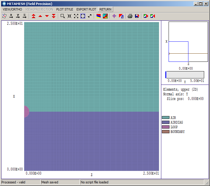
As in the 2D calculation, the goal is to find the self-inductance of a circular rod. The rod diameter is d = 2.0 cm and the loop diameter is D = 20.0 cm. The rod lies in the x-y plane and carries azimuthal current. To approximate an infinite space, the loop is located inside a box 100 cm on a side. To minimize solution time, the solution volume includes only the first quadrant in x-y and the region z >= 0.0. The top figure shows a detail of the mesh in the plane y = 0.0. The file Loop3D.CDF defines a filamentary circular loop carrying 1.0 A at radius 10.0 cm. The physical loop is assigned a relative magnetic permeability of MuR = 0.001. The resulting combination simulates a self-consistent surface current on the field excluding loop.
As described in Sect. 11.5 of the Magnum manual, the default boundary condition is that lines of B are parallel to surfaces. It applies at all surfaces of the solution space except the lower boundary in z. Nodes on this surface are marked with a unique region number in MetaMesh and asigned the fixed value of reduced potential Phi = 0.0 in the Magnum solution. The Dirichlet condition on the surface specifies that lines of B are normal to the surface. The region AIRDIAG shown in the figure is of special interest. It is a cylinder of radius 10.0 cm that extends over the full height in z. The inductance will be calculated by taking an integral of flux over its surface. Normally, the total magnetic flux over any solid body should equal zero. The convention in MagView is to omit any boundary facets. Therefore, the integral is performed only over the outer surface, giving the flux escaping from the cylinder.
|
|
Results
|
The solution takes only a few minutes. The analysis script Loop3D.SCR has the content:
*  NReg      RegName
*  =============================
*     1      AIR
*     2      AIRDIAG
*     3      LOOP
*     4      BOUNDARY
INPUT Loop3D.GOU
OUTPUT Loop3D.DAT
POINT 0.00 0.00 0.00
VOLUMEINT
SURFACEINT 2 -1
ENDFILE
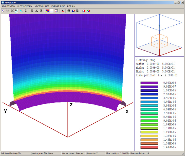
The lower figure shows a 3D view of the loop and diagnostic region surface. Values of |B| on the surface a included. The calculated magnetic flux density at the origin is Bz = 6.3607E-6 T, within 1.2% of the analytic value. The volume integral of field energy over one octant of the solution space is U/8 = 1.8522E-8. The total field energy is U = 1.4818E-7 J, implying a self inductance of 2.9636E-7 H. The integral of magnetic flux out of one forth of the cylinder surface is Phi/4 = 7.3889E-8 corresponding to a self inductance of 2.9556E-7 H. The values are within 0.7% of that calculated by the 2D high-frequency model.
|