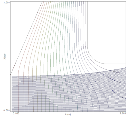
Trak can include contibutions of cathode temperature to the emittance of extracted electron beams. The theory of how the thermal energy of electrons emitted a hot cathode appears as an angular beam divergence is discussed in Sect. 10.3 of the Trak manual. This example reviews setup techniques. The upper figure shows the geometry. The cathode, focus electrode and emission surface are at -10.0 kV and the anode is at ground potential. The calculation is performed in the SCharge mode. The emission surface that covers the planar cathode has region number RegNo = 3. Space-charge limited emission for a cold cathode is controlled by the following command in the Trak input script HotCathodeTrak.TIN:
EMIT(3): 0.0000E+00 -1.0000E+00 5.0000E-02 2
The first two parameters (0.0 and -1.0) signal that the emitted particles are electrons. The third parameter is the distance from the physical cathode surface to the virtual emission surface, 0.05 cm (two element widths). At this spacing, the potential at the virtual emission surface is about 50-100 V. The final parameter is the number of model electrons to create per facet of the emission surface.
|
Results
|
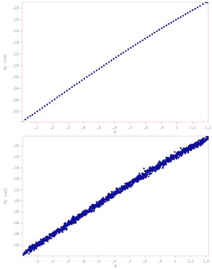
The cold-cathode calculation gives the model electron trajectories of the central figure. The initially-parallel beam diverges because of the negative lens effect at the extraction aperture. The space-charge-limited current is 1.432 A. The upper illustration of the lower figure (created with GenDist) shows the radial phase-space distribution of the exit beam. It follows a line of effectively zero thickness. The line is not straight because focusing forces in the gun do not vary linearly with r.
To model a hot cathode, the emission command was modified to
EMIT(3): 0.0000E+00 -1.0000E+00 5.0000E-02 2 1.0E4 0.2 20
There are three extra parameters. The number 1.0E4 is a source limit on current density. In this case, the number acts only as a placeholder and is set to a value much higher than the expected space-charge limit. The number 0.2 is the cathode temperature in eV. In order to calculate initial angles, it is important that this number be small compared to the electrostatic potential of the virtual emission surface. Finally, the number 20 is a statistical splitting factor. Each model particle is split into 20 independently-emitted sub-particles for a total of 1369 to give an accurate phase-space distribution. The bottom illustration in the lower figure shows the results. The phase-space distribution r-rp exhibits a The graph indicates an angular spread was about 0.005 radians. For comparison, the predicted angular spread is on the order of (kT/Te), where Te is the exit energy in eV. Taking kT = 0.2 and Te = 1.0E4, the value is about 0.0045 radians.
|
|
Comments
|
For comparison, the same calculation performed with the 3D OmniTrak code: cathode_temp_omnitrak.html.
|