My original intent was to write an article to show when it is necessary to use an eddy-current code to find time-varying magnetic fields and when a static field code like Magnum is sufficient. As a preliminary, I thought it would be useful to review how eddy currents affect magnetic fields in single wires. This tutorial has two purposes:
- Document useful general results on the effective resistance and ohmic losses in wires at high frequency.
- Show how to set up calculations of magnetic field distributions in wires with the two-dimensional code Nelson.
To start, let's review some basic equations for a long wire with cross-section area Aw (m2) and conductivity σ (S/m). At low frequency, the current density is uniformly distributed across the wire and the resistance per length given by Eq. 1. If the wire carries an alternating current Io cos(2πf t) at frequency f, Eq. 2 gives the time-averaged power dissipation.At high values of f, the magnetic field associated with the current flow is inhibited from penetrating the metal wire, concentrating the current density near the wire surface. The effective effective cross-section area of the wire is therefore smaller than Aw, increasing the resistance per length and the ohmic power loss for a given current. The penetration distance for magnetic fields, called the skin depth, is given Eq. 3. The quantity μ is the magnetic permeability, given by μ = (1.257E-6) μr, where μr is the relative magnetic permeability. The relative permeability equals 1.0 for most wire metals.
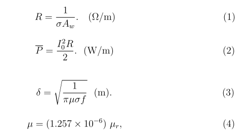
The skin depth allows us to define the high and low-frequency regimes. For a circular wire of radius rw, Eq. 4 gives the condition for enhanced ohmic losses. In the following calculation, we'll use the example of a circular copper wire 1.0 mm in radius. The conductivity of copper is σ = 5.814E7 S/m. Using Eq. 3, the frequency corresponding to ? = 0.5 mm is 17.4 kHz. For a wire area Aw = 3.142E-6 m2, Eq. 1 gives the steady-state resistance R = 5.474E-3 ?/m. For a drive current amplitude I0 = 1.0 A, the low-frequency power loss is P = 2.738E-3 W/m.
The program Nelson finds field magnetic distributions in the frequency domain?? all quantities (including drive currents) vary harmonically at the same frequency. The input files to define the mesh and to control the calculation are circular.min and circular.nin. Figure 1 shows the mesh with dimensions in millimeters. The wire extends an infinite distance out of the page. The large air region was included so that the calculation could easily be modified for non-circular wires -- the distant boundary has little effect on the magnetic fields inside a wire.
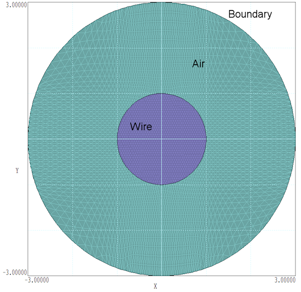
Figure 1. Mesh for the Nelson circular wire calculation.
In the Nelson control script circular.nin, the boundary is a surface of fixed vector potential (flux conserving boundary) and the air region has ?r = 1.0 and ? = 0.0 S/m. The copper wire has ?r = 1.0, ? = 5.814E7 S/m and a drive current I0 = 1.0 A at a phase of 0.0?. The calculation of eddy currents in the wire uses the multistage, self-consistent method described in Chap. 4 of the Nelson manual. Figure 2 shows lines of B. At low frequency, |B| inside the wire increases linearly with distance from the axis, consistent with uniform current density. At high frequency, the magnetic flux density is concentrated on the surface.
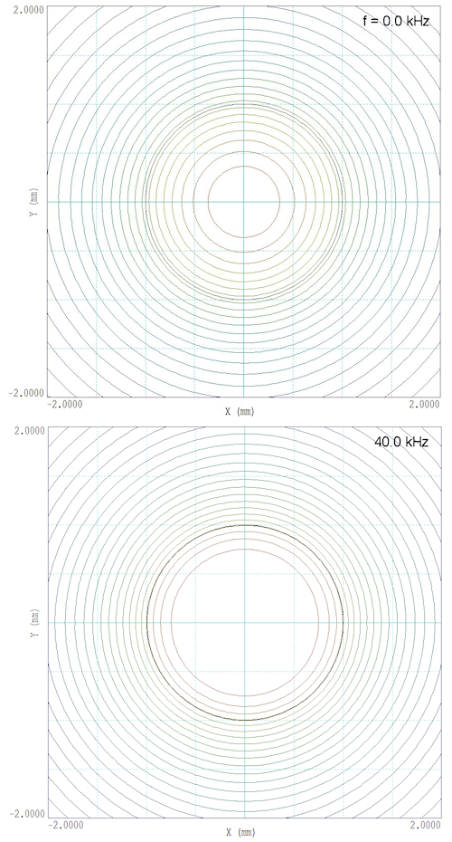
Figure 2. Lines of magnetic flux density in and around a circular copper wire at low and high frequency.
To make a quantitative comparison, we can use the automatic volume integral in the Nelson Analysis menu to find the total power dissipation per length along z. Results of calculations at several frequencies are plotted in Fig. 3. The theoretical steady-state value is shown as a dashed line. As expected, power losses increase significantly in the range 10-20 kHz. At high frequency, the current is confined to a thin layer on the wire surface. In this case. the power loss increases approximately as ?f, proportional to 1/?.
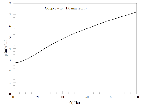
Figure 3. Power dissipation per meter in a copper wire of radius 1.0 mm as a function of frequency with a drive current amplitude of 1.0 A.
It is important to recognize that the numerical results for the 1.0 mm copper wire may be applied to circular wires of any diameter or composition. It is not necessary to repeat the calculation for each special case. The strategy is to recognize scaling laws and to incorporate them into a universal curve. As an example, the green line of Fig. 4 plots the power level relative to the steady-state value as a function of the ratio of the wire dimension to the skin depth. There are two advantages to applying scaling laws:
- Generality ? the graphed data may used to determine the effective resistance of any circular wire.
- Identification of trends ? it's evident that the power loss is proportional to 1/? at high frequency.
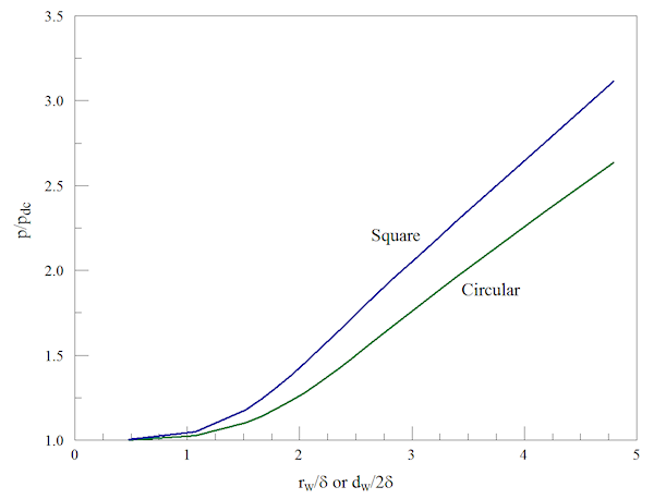
Figure 4. Universal curve for high-frequency wire resistance, power relative to the steady-state value plotted as a function of the wire dimension normalized by the skin depth. Circular and square wire cross sections.
As an example, suppose we have a 1/8"' diameter stainless steel rod and we want to find the frequency limit such that the power loss is no more than 50% of the low-frequency value. An inspection of Fig. 4 shows that ? must be greater than rw/2.5. With ? = 1.240E6 S/m and rw = 1.59 mm, the frequency corresponding to ? = 0.636 mm is f = 503.7 kHz. To check the result, I set up another Nelson calculation with modified wire radius and conductivity. For I0 = 1.0 A, the predicted steady-state power dissipation is 50.77 mW/m. The Nelson calculation gives 50.77 mW/m at f = 1.0 Hz and 76.28 mW/m at 503.7 kHz. The ratio of the two power levels is 1.50.
The results for circular wires could have been derived analytically with some effort. The true advantage of a numerical approach is that complex shapes are no more difficult to handle than simple shapes. To illustrate, I set up a run for square copper wires by changing the shape of the wire region in the Mesh input file. I used a wire with side lengths D = 2.0 mm. Figure 5 shows lines of B at high frequency. The universal power dissipation curve for square wires is plotted as the blue line in Fig. 4. For more information on Nelson, please see http://www.fieldp.com/nelson.html.
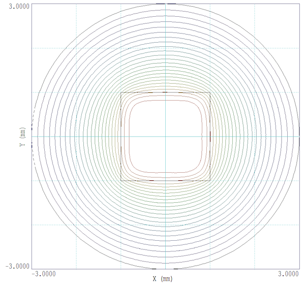
Figure 5. Lines of magnetic flux density in and around a square copper wire at 40 kHz.
LINKS
