This note gives a capsule summary of the rules the govern common boundary conditions in WaveSim. In 2D electromagnetic solutions (either analytic or numeric), the standard approach is to divide waves into two polarity classes. In WaveSim, we designate the classes as E and H type waves:
- In an E wave, the electric field vector is normal to the solution plane. In a planar solution (variations in x and y with infinite length in z.), the electric field has the single component Ez and the magnetic field has components Hx and Hy. In a cylindrical solution, the solution plane is r-z. In this case, the field components are E?, Hz and Hr.
- In an H wave solution, the magnetic field vector is normal to the solution plane. The field components in a planar solution are Hz, Ex and Ey. In cylindrical geometry, the components are H?, Ez and Er.
Absorbing layers usually occur on the boundary of the solution volume. The layer often covers the full boundary to simulate the free-space condition. Sometimes, the layer covers a portion of the boundary, such as the termination of a coaxial transmission line. The same approach applies to both E and H type solutions. Leave the outer boundary of the layer unspecified and assign absorbing properties by setting the imaginary part of the electric permittivity (E type solution) or magnetic permeability (H type solution) using the formulas in Table 6 of the WaveSim manual. In the new version of program, you can let the program do the work by employing the AbsLayer command.
The other common boundary is a perfectly-conducting metal. Here, we must differentiate between external and internal boundaries. The term external refers to the boundary of the solution volume (which need not fill the entire solution box). A familiar instance of an external metal boundary is the wall of a resonant cavity. The approach depends on the mode type:
- H type. No user effort is necessary. All unspecified external boundaries act like metal walls.
- E type. In 2D solutions, the electric field is parallel to the boundary and must therefore equal zero. In this case, trace the metal boundary with a line region and set its properties with the Reflect command (i.e., Ez or rEθ = 0.0).
When defining internal metal objects (e.g. scattering from a metal extrusion), we must ensure the proper boundary conditions for E and H on the object surface. The same procedure applies for both E and H modes: set a very large value for the real part of the relative dielectric constant. This ensures that the component of electric field parallel to the boundary is zero.
Mu(5) = 1.0
Epsi(5) = 1.0E12
Figure 1 shows lines of electric field for an H wave scattered from a metal rod. Note that the electric field lines are everywhere normal to the surface.
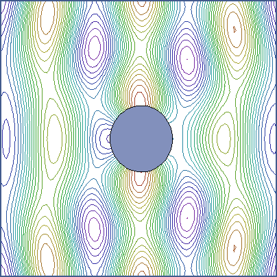
Figure 1. H type wave scattered from a metal rod.
There is an alternative that works only for E waves:
Reflect(5)
In the case, the total electric field is parallel to the boundary so we can set it identically equal to zero. There is an important precaution for using the Reflect command for either external or internal boundaries.? The condition affects nodes of the solution volume; therefore, we must be sure that nodes common to two regions are set properly. Because of the over-write conventions, regions that will assume the Reflect condition must appear toward the bottom of the Mesh script.
LINKS
