Our code packages have extensive features and attack difficult physics solutions. It would be unrealistic to imply that anyone could learn a package by spending an afternoon pushing buttons. On the other hand, although the codes are big, need they be beyond your understanding and control? Are they unapproachable black boxes that require complete faith?
The purpose of this article is to answer "no" and to illustrate steps you can take to tame the programs. The strategy is to follow the same type of procedure we do. When we complete a 3D solution package, it seems inconceivable that something that complex could ever give the right answer. And "inconceivable" wins the day, because the programs never work the first time. We begin a testing sequence, starting with a simple, incontrovertible solution. We identify and fix the problems, make sure we get the right answer, and then move another rung up the ladder.
When you are ready to create your own solutions, start with a simple geometry where you know the answer. If the results don't meet your expectations, find out why. With a few examples, you will learn a lot about the program and the limits of numerical techniques in general. To illustrate, I will work through a test electrostatic solution with HiPhi, comparing the answers to textbook results. In the process, we will check the numerical accuracy and review the calculation of capacitance.
The figure below shows the geometry, an ideal spherical capacitor with outer electrode at r0 = 5.0 cm, inner electrode at ri = 2.0 cm and an intervening dielectric with εr = 2.7. The element width is about 0.2 cm. The closed sysyem avoids issues with boundaries, an unavoidable feature of finite-element solutions. The mesh is created in MetaMesh by filling the solution volume with the outer wall, cutting out the spherical volume of the dielectric, coating the outer surface so that all shared nodes are associated with the outer wall, and then adding the inner sphere. The inner electrode has potential V0 = +1.0 V and the outer surface is grounded. With the relatively large element size, the HiPhi solution takes only 15 seconds.
The file sphere.scr is an analysis script for PhiView and has the following content:
* File SPHERICAL_CAPACITOR.SCR
* Copyright, Field Precision, 2008
OUTPUT Spherical_Capacitor
INPUT Spherical_Capacitor.HOU
* Check absolute values at two points
POINT 3.0 0.0 0.0
POINT 4.0 0.0 0.0
* Calculate global field energy to find capacitance
FULLANALYSIS
* Determine induced charge and compare capacitance values
REGION 1
REGION 3
ENDFILE
The predicted variation of electric field between the electrode surfaces is:
Er(r) = (V0/(1/ri - 1/ro)
where all quantities are in SI units. Here are the code results at the two points:
Radius   Er(analytic)    Er(code)      Difference
(cm)       (V/m)         (V/m)
================================================
0.03       37.037        37.186         0.402%
0.04       20.833        20.850         0.082%
It is comforting that the absolute agreement is very good. As in any numerical calculation, the agreement is not perfect. You can improve the accuracy by reducing the element size in the MIN file to 0.1 cm. The price to pay is that the run time increases by more than a factor of eight. In any numerical calculation, you must decide the accuracy you need and balance it against the run time you can spare.
The equation for the capacitance between concentric spheres is
C = 4π εrε0/(1/ri - 1/ro).
In this case, the predicted value is C = 1.0014 × 10⁻¹¹ F. There are two ways to find the capacitance of a two-electrode system in PhiView: 1) find the global field energy and use the formula U = CV2/2 or 2) find the charge on the electrode surface by calculating the normal component of electric field. For the example, the FULLANALYSIS command yields the energy U = 4.9711 × 10⁻¹² J. The capacitance is therefore C = 9.9423 × 10⁻¹² F, about 0.72% lower than the ideal value. The main cause of the difference is probably the volume difference of the inner electrode, which is a faceted shape rather than a perfect sphere. Again, the results will improve considerably with smaller element size. The induced charge calculation gives -1.02134 × 10⁻¹¹ coulomb on the inner electrode and 1.00928 × 10⁻¹¹ coulomb on the outer. The implied capacitance values differ from the theoretical value by +2.1% on the inner and +0.93% on the outer. The induced method is generally less accurate than the energy method because it involves local field interpolations close to electrodes rather than an average of interpolations through the medium. Note that the accuracy is better on the outer electrode because the surface has a larger number of facets and more closely approximates a sphere.
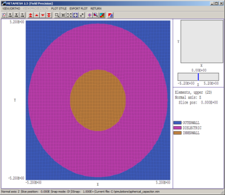
Capacitance of concentric spheres.
LINKS
