A trial user posed the problem related to the system of Fig. 1. A three-phase power line parallels a transport pipe for natural gas. The line and pipe are buried in the earth. What would happen if one of the wires in the power line shorted to the earth? With regard to a gas explosion, what is the current carried by the pipe, and is there a significant electric field inside? The trial user specified a peak current of 42 A at frequency 50 Hz at the shorting point and gave conductivity values of σ = 0.0066 S/m for the earth and 0.0039 S/m for the concrete. Because the problem involved time-varying currents and applied to a long pipe, he requested a trial of the 2D Universal BField Toolkit. Although he generated carefully-prepared input files for the Pulse program, it was not at all clear what the results meant.
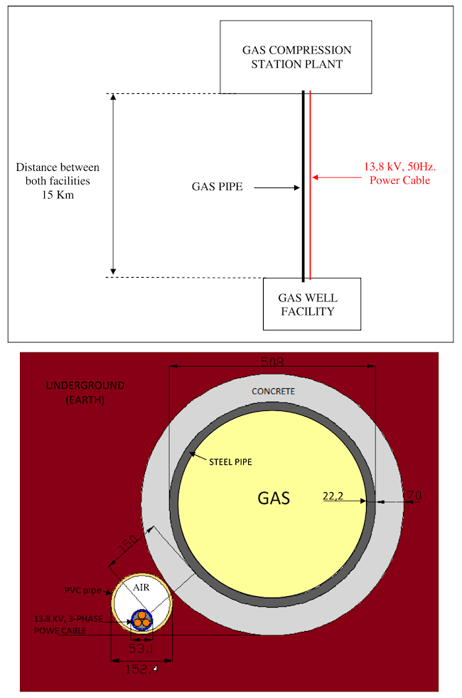
Figure 1. Definition of calculation.
I determined that the Pulse program for the calculation of time-dependent magnetic fields and inductive electric fields is not applicable. Let's see why. The wavelength of electromagnetic radiation in air at 50 Hz is 6 million meters. Even if the ground had a significant relative dielectric constant, the wavelength is large even compared to the 15 km length of the pipe. Furthermore, the skin depth for magnetic-field penetration into the surrounding medium is over a km. Therefore, the role of inductive electric fields is negligible. Voltage differences arise from the flow of real current through the conductive media. The system is essentially a resistive voltage divider, that can be modeled with an electrostatic code like HiPhi.
Before getting involved in numerics, it's useful to ask what is the worst possible scenario. At some point, all the current from the short-circuit makes its way through the earth and concrete to the pipe, where it travels several kilometers back to the station plant. If the return current is distributed uniformly over the pipe cross-section, the resistance per length for a conductivity σ is
r = 1/σ*A,
where the cross section area A is 2πR2. Values σ = 8.2E4 S/m, R = 0.25 m and R = 0.022 m imply a resistance per length of 3.5E-4 Ω/m. For a current of 40 A, the maximum field inside the pipe is only 13 mV/m, well below the level for corona. Actually, the field is even less than this value. The skin depth in steel is
δ = sqrt[1/(π σ μr μ0 f).
For μr = 1500 and f = 50.0 Hz, the skin depth is only δ = 6.38 mm, implying good shielding. I could have employed Pulse for this type of calculation, but it is probably not worth detailed simulations for such small field values.
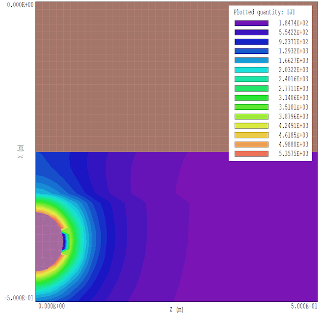
Figure 2. Plot of current-density amplitude near the short-circuit. The discontinuity shows the surface of the concrete.
On the other hand, it is useful to perform numerical calculations to see what type of voltages occur outside the pipe and the length scale for collection of all current on the pipe. I set up an electrostatic solution using HiPhi in a large solution volume (a cube 20 m on a side) with a steel pipe of radius 0.25 m inside a concrete pipe of radius 0.32 m. Both pipes ran the length of the solution volume along z. The bulk of the solution volume (earth) was a conductor with σ = 0.0066 S/m while the concrete pipe had σ = 0.0039 S/m. The steel pipe was an equipotential region at φ = 0.0. I represented the source of short-circuit current as a fixed-potential sphere of radius 0.05 m at a distance 0.4 m from the pipe center. I set the sphere potential at 1.0 V in an initial solution and used the automatic capability of PhiView to perform a surface integral of current collected by the pipe. I then adjusted the source potential to give a collected current of 42 A. At the adjusted potential of 40 kV the peak electric field on the source surface was about 8000 V/cm. It is probable that sparks and breakdown would be localized to the immediate region of the short circuit. Figure 2 shows a spatial plot of current-density amplitude near the short circuit in the plane y? = 0.0 m. Figure 3 shows a scan of current density along the surface of the pipe on the side facing the source. Despite the low conductivity of earth, most of return current was collected by the pipe within 0.5 m of the short-circuit point.
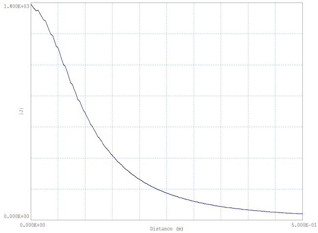
Figure 3. Scan of |J| along the surface of the pipe facing the source.
LINKS
