Finite-element electrostatic field solutions apply to finite volumes. One of the most common difficulties that new users of EStat and HiPhi face is how to deal with the boundaries of the solution volume. The challenge is to set boundary properties for the best representation of the physical system.
To illustrate, consider the fields generated by the two electrodes shown in Fig. 1. Your first impulse might be to say that I'm only interested in the electrodes, so I just won't do anything about the boundaries. In this case, the boundaries assume the special Neumann condition, the natural assignment for a finite-element solution. As shown in the left-hand figure, equipotential contour lines are normal to the boundary and electric fields are parallel. What can we say about this solution?
- The extended Neumann boundary boundary slows convergence of the solution. This is a particular concern in HiPhi.
- The boundaries force the contours to be normal, so that the region about the electrodes does not act like an infinite free space. Instead, the solution corresponds to an infinite array of electrode pairs in x and y.
- The electric field lines make a right-angle bend in the corners, so that the solution is not entirely physical.
We need to consider two things for a complete solution definition: 1) the primary region of interest and 2) the environment around the solution. In this case, the region of interest is probably the high-field space between and near the electrodes. There are different possibilities for the surroundings.
- Suppose the electrodes extend a long distance out of the page and we are looking at a cross-section well removed from electrical connections. In this case, the electrodes are surrounded by a large free-space volume where the potential approaches ground potential at a large distance. Here, we could enlarge the solution volume at relatively coarse resolution and set the fixed-potential condition φ = 0.0 over the entire boundary. This choice eliminates the bending effect of the nearby Neumann boundaries. For reasonable choices, the exact size of the solution volume would have little effect on fields in the region of interest.
- Suppose there are extended connecting structures that we choose not to represent. The structures above the solution are at the potential of the top electrode and those below at the potential of the bottom electrode. Therefore, there is an approximately uniform vertical electric field far from the electrodes. In this case, we set fixed potentials on the top and bottom boundaries, as shown in the right-hand figure. We might also increase the solution size in the horizontal direction to reduce the effect of the left and right-hand Neumann boundaries.
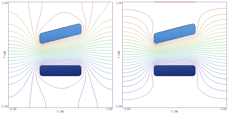
Figure 1. Electrostatic solutions with different choices of boundary conditions.
The implication is that you have to think about the boundaries of each solution and plan accordingly. This makes some users resentful. Why can't the program figure it out? The point is that whenever you set out to make a mathematical representation of a physical system, you are already making decisions about limiting the calculation. For example, there's a beer can lying in a field in Davenport, Iowa that will have a non-zero (albeit small) effect on your solution. Would you include it? The bottom line is that there is no such thing as a computer simulation (i.e., a perfect solution that includes every possible effect at a location). Each numerical solution reflects a multiplicity of filtering decisions made by the user.
LINKS
