In the tutorial Designing permanent-magnet solenoids with PerMag, I discussed how permanent magnets with radial magnetization could be used to generate a solenoid field. An annular magnet with pure radial magnetization is impossible to fabricate with modern high-energy-product materials. Instead, it must be approximated with a set of Ns wedge sectors, each with linear magnetization. There are two questions to address for such an assembly:
- How does sectoring reduce the achievable solenoid field? In other words, how does the value of the peak magnetic flux density in the solenoid vary with Ns?
- How many sectors are necessary for good azimuthal uniformity of the field at the working radius?
The calculations described in this article address the issues and demonstrate some setup techniques for Magnum, our three-dimensional magnetic field code.
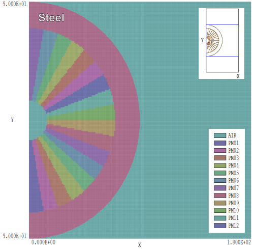
Figure 1. Half-section of a 36-sector permanent magnet — view of the mesh in the x-y plane. Dimensions in mm.
Figure 1 shows the geometry of the test calculation. The full assembly consisted of two annular permanent magnets connected by a steel flux conductor. The magnets had approximately radial magnetization with opposite polarities. Each magnet had inner radius 15.0 mm, outer radius 70.0 mm and 50.0 mm axial length. The upper magnet extended over the axial region 15.0 mm ≤ z ≤ 65.0 mm. The steel shield with inner radius 70.0 mm and outer radius 90.0 mm extended from z = 0.0 mm to z = 65.0 mm. The annular permanent magnets had Br = 1.4 tesla and were divided into 36 azimuthal 10? sectors. The element resolution was 1.0 mm in the magnet volume with a surrounding volume at coarse resolution for fringing fields. The Magnum calculation had the following features:
- I reduced the run time by performing the calculation in the half-space z > 0.0 mm with the symmetry condition B(parallel) = 0.0 at z = 0.0 mm. To define the boundary at z = 0.0 mm, I set a condition of fixed reduced potential, φ = 0.0.
- With field perturbations in the y direction, the condition B(normal) = 0.0 was automatically satisfied at x = 0.0 mm. The boundary was implemented by simply limiting the mesh to x ≥ 0.0 mm.
- Each of the 18 sector parts in the half space x ≥ 0.0 mm was associated with a region. In Magnum it is possible to assign individual region values of Br and the magnetization direction.
- It was not necessary to employ conformal fitting of elements to achieve good accuracy for two reasons: a) adjacent sectors differed only in their direction of magnetization so there were no strong boundary processes and b) the fields of interest near the center of the solenoid were well removed from the sector boundaries.
I changed the effective number of sectors through assignment of magnetization directions in the Magnum input files. For Ns = 36, each of the 18 permanent magnet regions had a different value of the magnetization angle, -85°, -75°, -65°, ... , +75°. For Ns = 12, a single angle was assigned to a group of 3 regions. For example, magnets 1, 2 and 3 had angle -75°.
Field reduction as a function of number of sectors
Ns    Bz(0,0,0) Bz/Bz
 6    1.3130    -4.52%
12    1.3593    -1.15%
18    1.3680    -0.53%
36    1.3732    -0.14%
The three-dimensional calculations gave the values for the axial magnetic field at the midpoint of the magnet shown in Figure 2. As expected, the division into sectors with linear magnetization reduced the attainable field. For an accurate determination of the relative change, I needed a field value for Ns = ∞. A calculation using the PerMag code for a cylindrical assembly with perfect radial magnetization gave Bz(0,0,0) = 1.3810 tesla. Although the value was very close to the three-dimensional results, it was not accurate enough to determine the small relative error for Ns = 36. The figure below illustrates the standard interpolation technique to resolve the problem. The field values are plotted versus 1/Ns. The zero value on the abscissa corresponds to an infinite division of sectors. The strategy is to fit the values with a second-order polynomial and to identify the intersection with the axis. A negligibly small linear term confirms that there is no systematic error in the calculation. The projected value for a perfect radial magnet was 1.3751 tesla (a difference of 0.4% from the PerMag calculation). The relative reductions shown in the table were calculated from this value. The implication is that sectoring gives only a small reduction in the central field.
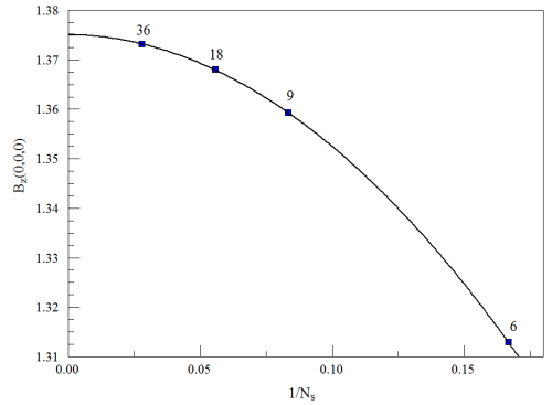
Figure 2. Magnetic field at the magnet center [0.0, 0.0, 0.0].
Azimuthal variations of magnet structure can cause variations in the solenoid field. We expect that the amplitude of field variations increases with radius and with a smaller number of sectors. To determine azimuthal variations of the calculated field, I generated data with the GENSCAN script command of the MagView postprocessor. In response to the command, the code performs a set of second-order interpolations at listed positions in the solution space. In this case, I used a spreadsheet to prepare a list of 180 coordinates at a circle in the x-y plane at axial position z = 10.0 mm. I performed calculations at radii of 2.0, 5.0 and 10.0 mm. The results at r = 10.0 mm are plotted in Figure 3. The plot shows Bz as a function of angle and Ns. For large values of Ns, the variations are obscured by numerical noise. The standard deviation of Bz in the Ns = 36 curve is ?0.00073 tesla. A coherent variation is perceptible only at the lowest number of sectors (Ns = 6). In this case, the coherent field variation is only ? 0.2%. Variations were undetectable for any number of sectors at r = 2.0 mm and r = 5.0 mm. The conclusion is that field variations associated with magnet sectoring are quite small for Ns > 9.
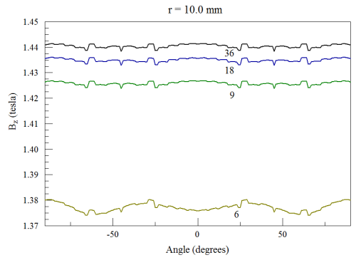
Figure 3. Variation of Bz at a radius of 10.0 mm in the x-y plane at z = 10.0 mm as a function of angle and the number of magnet sectors.
LINKS
