In my role of writing and maintaining the Trak and OmniTrak codes, I often think about electron-beam extractors. The critical issues are limits on current density and beam coherence. Both may be affected by the temperature of thermionic cathodes. The topic was studied theoretically almost a century ago by Langmuir [ I. Langmuir, Phys. Rev. 21, 419 (1923)] and other authors because of its relevance to vacuum-tube technology. But like many results in collective physics, the equations are complex so that limiting conditions must be applied to find analytic solutions. Although the Langmuir results are often cited, they are seldom used. To generate useful information for use in my codes and for other designers, I carried out new studies using numerical techniques. The advantage is that direct numerical solutions address a broad range of parameters without the need for limiting approximations. I applied scaling principles to create a set of universal curves that can be applied to any electron or ion source. I summarized the results in a paper that you can download at this link: Cathode thermal effects in one-dimensional space-charge-limited electron flow.
This article and following ones review the essential physics of the paper and display the results in an easily accessible form. The following topics are addressed:
- This article reviews limits on electron flow set by space-charge effects (the Child law).
- The second article shows how to create model particles that follow the Maxwell-Boltzmann distribution, a useful technique for those involved in numerical simulations
- The third article shows how to employ scaling relationships to derive general conclusions from specific numerical calculations. It summarizes conclusions of the paper including universal curves for electron emission.
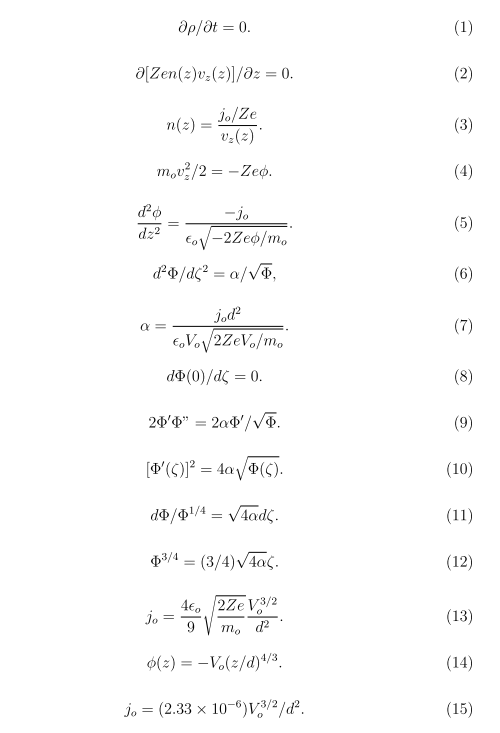
As a preliminary, it's useful to review the basis for space-charge limitations on electron flow. For a more complete discussion, see Sect. 5.2 of my book Charged Particle Beams which is available for free download at http://www.fieldp.com/cpa.html. The Child law determines the maximum current density that can be carried by charged particle flow across a one-dimensional extraction gap. The limit arises from the longitudinal electric fields of the beam space-charge. Figure 1 shows the geometry, a one-dimensional acceleration gap of width d and applied voltage V0. In this case, quantities vary only in z and the gap has infinite extent in x and y. Of course, real extractors have finite dimensions. Such geometries must be handled by numerical codes like Trak (cylindrical) or OmniTrak (sheet beams and general 3D). Charged particles with low kinetic energy enter at the grounded boundary. The particles have rest mass m0 and carry charge +Ze. The particles leave the right-hand boundary with kinetic energy ZeV0. The following assumptions simplify the calculation of self-consistent flow:
- Particle motion is non-relativistic (eV0 ≪ m0 c^2).
- The source on the left-hand boundary supplies an unlimited flux of particles. Restrictions of flow result entirely from space-charge effects.
- The transverse magnetic force generated by current across the gap is small compared to the axial electric force.
- Particles flow continuously — the electric fields and space-charge density at all positions in the gap are constant.

Figure 1. Geometry for the calculation of space-charge-limited flow across an infinite planar acceleration gap.
The steady-state condition means that the space-charge density, ?(z), is constant in time (Eq. 1). Combining Eq. 1 with the conditions of conservation of particles gives Eq. 2. The equation implies that the current density, equal to Zen(z)vz(z), has the same value at all positions in the gap. This constant value is designated j0. The density of particles as a function of position is given by Eq. 3. If we take the electrostatic potential equal to zero at the particle source, the velocity and potential are related by Eq. 4. The density may be expressed as a function of φ by inserting Eq. 4 into Eq. 3. The result can then be substituted in the one-dimensional Poisson equation to give Eq. 5
Equation 5 can be solved with appropriate boundary conditions to find the self-consistent variation of ?(z). The result may substituted in Eq. 3 to find the variation of particle density.
Equation 5 may be written in a more succinct form by introducing the dimensionless variables ζ = z/d and?? = -Φ/V0. The result is Eq. 6 where the parameter α is given by Eq. 7. Two of the boundary conditions are Φ(0) = 0 and Φ(1) = 1. A third condition is necessary to define a unique solution. For space-charge-limited flow, the condition is that the electric field at the source equals zero (Eq. 8). The condition may be understood by inspecting inspecting Figure 2. The figure shows a set of possible solutions of Eq. 5. If the available current density from the source is low, then a solution like that of curve A results. The potential variation is almost the same as the vacuum solution with no contribution from space-charge?? the electric field is nearly uniform across the gap. With higher source flux there is more positive space-charge in the gap. Curve B shows the potential with space-charge contributions. The average potential in the gap is higher and the electric field at the source is lower. Suppose we continue raising the flux until the electric field at the source approaches zero (curve C). Then, particles with low kinetic energy are just able to leave the source. Higher gap flux is impossible?? it would result in a negative electric field at the source that repels entering particles. The flux of particles across the extraction gap saturates at the level where Φ'(0) = 0, independent of further increases in the available flux from the source. At this point, we say that the extraction gap passes from source-limited flow to space-charge-limited flow. Following articles will clarify the physical basis of the transition.
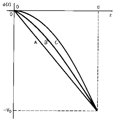
Figure 2. Axial variation of electrostatic potential in an infinite planar acceleration gap. (A) Low beam current. (B) Moderate beam current. (C) Space-charge-limited beam current.
Equation 6 can be solved by multiplying both sides by 2Φ', where Φ' = dΦ/dζ. The left-hand side of the resulting Eq. 9 is an exact differential of Φ2. Integrating both sides of Eq. 9 from the source to position z and applying the boundary conditions gives Eq. 10. This equation may be rewritten as Eq. 11. Both sides of Eq. 11 can be integrated — the result is Eq. 12. The boundary condition Φ(1) = 1 implies that α = 4/9. Substituting the definition of α from Eq. 7 and solving for the current density gives the Child law for space-charge-limited extraction, Eq. 13.
For space-charge-limited flow, the electrostatic potential varies with position as Eq. 14 (curve C of Fig. 2). Equation 13 states that for a given gap voltage and geometry, the current density is proportional to the square root of the charge-to-mass ratio of the accelerated particles, ?(Ze/m0). The allowed current density of electrons is roughly 43 times higher than that of protons. In electron and proton extractors with the same values of d and |V0|, the densities are the same but the electrons move faster by a factor ?(mp/me) . For reference, the Child limit for non-relativistic electrons is given in Eq. 15. For V0 in volts and d in centimeters, the units of Eq. 15 are A/cm?.
LINKS
