Thin sheets are the bane of finite-element calculations. Large disparities in scale lead to bad meshes and bad answers. The issue often arises in magnetic-shielding calculations where thin layers of iron or mu-metal are used to reduce the field level around sensitive instruments like photomultipliers. In such cases, it is useful to employ scaling principles rather than to take a literal approach. You can avoid headaches creating the mesh and often achieve better accuracy.
To illustrate, we will use the example of a hollow iron sphere immersed in a uniform magnetic field from J.D. Jackson, Classical Electrodynamics. Figure 1 shows the geometry in an r-z plot. (Note that the figure does not show half the sphere — It shows the entire sphere in r and z coordinates.) The sphere has outer radius ro and inner radius ri. If consists of an iron-like material with relative magnetic permeability μr. The field far from the sphere has the uniform value Bz = Bo. The analytic solution shows that if μr ≫ 1, then the field inside is uniform and axial. The ratio of the field inside the sphere to the far field is
Bi/Bo = (9/2*μr)/(1 - ri^3/ro^3). [1]
Assuming the thickness of the sphere is small compared to the average radius, taking Δr = r0 - ri, and doing a binomial expansion, we can write the ratio as:
Bi/Bo = (3*ro)/(2*μr*Δr). [2]
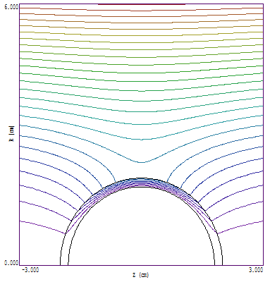
Figure 1. Hollow iron sphere in a uniform magnetic field.
We can run a PerMag solution with cylindrical symmetry to check the result. We will place a sphere of radius ro = 2.0 cm inside a large solution volume, a cylinder of radius 10.0 cm and length 20.0 cm. We want to set things up so there is a uniform field Bz = 0.050 tesla (500 G) in the absence of the sphere. We use the following trick:
- The left and right boundaries have the Neumann condition (normal B field), the natural boundary condition in PerMag.
- Set the vector potential on the axis to r*Aθ = 0.0 (Dirichlet condition)
- Set the vector potential on the outer boundary at R to rAθ = Bo*R^2/2 = 2.5E-4 (Dirichlet condition).
We confirm the technique by making an initial run with the iron set to μr = 1.0
In the first calculation, the inner radius of the sphere is ri = 1.95 cm, corresponding to thickness 0.05 cm. To resolve the shell, we use a small local element size of 0.025 cm. In this calculation, the calculated internal field is 1.187E-3 tesla, close to the theoretical prediction of 1.200E-3 tesla.
It's relatively easy to use very small elements in the 2D PerMag code, but it would be quite difficult and time consuming to model the thin shell with the 3D Magnum code. As an alternative, note that Eq. 2 involves the product of μr*Δr. What if we doubled the thickness of the shell and halved the value of μr? We should get about the same answer as long as Δr ≪ ri. In other words, we are simplifying the solution by applying a scaling relationship, a familiar approach in pre-computer engineering. If we use a thickness Δr = 0.10 cm and μr = 1250, the calculated field inside the shield is 1.218E-3 tesla. A thickness Δr = 0.15 cm with μr = 833.3 gives 1.2492E-3 tesla, about a 4% error.
As a general rule, in a 2D or 3D magnetic shielding calculation, you can substitute a thicker sheet with reduced μr as long as the actual and adjusted sheet thicknesses are small compared to the scale size of the volume being shielded. It is important to note that the procedure is invalid if parts of the shield become saturated. This condition violates the assumption of linearity underlying the scaling relationship. A related question is how do you know if the shield is saturated? Do a calculation with a reasonable fixed value of μr and check if B exceeds the saturation value Bs over a significant volume of the material. The saturation field for iron is about Bs = 2 tesla, and is much lower for materials like mu-metal.
If you want to run the Permag example, here are links to the input files:
shieldscaling.min
shieldscaling.pin
LINKS
