Recently I received two customer questions about strategies in our thermal programs TDiff (2D) and HeatWave (3D). The first was how to represent the effect of absorbed incident radiation. The assumption is that the user knows the properties of the radiation and the emissivity of the surface. In other words, how do we represent a known incident thermal flux, q(x,y,z) W/m?. Although both thermal codes model specified volumetric sources Q(x,y,z) W/m?, there isn't a direct method to specify an area source. The figure illustrates the simple resolution. Here, the surface of the material object is either on the boundary of the solution volume or is adjacent to a region with very small thermal conductivity (effectively a vacuum). The arrow indicates thermal radiation incident from outside the solution volume. We add an additional layer of thickness D. The value of D should be comparable to or larger than the local element size, but much smaller than the scale size of the object. We then assign a volumetric source within the new region such that
Q(x,y,z) = q(x,y,z)/D
For dynamic solutions, the layer should have a high thermal conductivity so that energy is transferred quickly to the material object. Furthermore, the product ρCp should be relatively small so that the layer does not affect the energy balance. The figure shows an alternate approach when radiation comes from a single direction. In this case, we can use a uniform volumetric source Q0 and vary the thickness D. If θ is the angle between the surface normal and the radiation direction, then the thickness should vary as cos(θ).
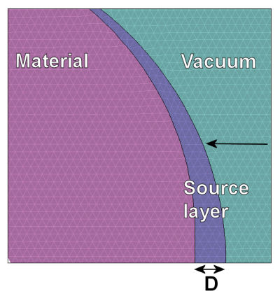
Surface layer to represent incident thermal radiation.
The second question is how to model the effect of a very thin layer of material. The thickness D is much smaller than the scale size of other objects, so it would be difficult to create a mesh that is a literal representation. As in previous blogs, scaling relationships come to the rescue. Suppose we increase the thickness of the layer by a factor M > 1.0. The width MD should be consistent with a reasonable element size but small compared to the size of macroscopic objects. In this case, the thermal solution would be approximately correct if we make the following changes to the material properties of the layer:
<
p>
k →
M*k
ρCp → ρCp/M
The first relationship ensures that thermal flux through the layer for a given temperature differential is unchanged. The second relationship specifies that the thermal inertia of the thicker layer is the same as the original one.
LINKS
