You can save and load plot views in our two-dimensional TriComp field programs (EStat, PerMag, EMP, Nelson, TDiff, Pulse, RFE2 and WaveSim). In the interactive environment, the Save view command generates a formatted text file FPrefix.FPV where FPrefix is a descriptive name assigned by the user. The file contains the complete set of plotting parameters. This excerpt illustrates the format:
Program: TriComp
PlotStyle: Spatial
Outline: ON
Grid: ON
Scientific: OFF
FixedPoint: OFF
Vectors: OFF
XGMin: 3.500000E+00
XGMax: 9.000001E+00
...
The file contains all necessary parameters to reconstruct spatial plots (in the z-r or x-y planes). The file includes the following information for spatial plots:
- Style information, like whether to display a reference grid, element outlines or field vectors.
- Boundaries of zoomed views
- The plot type (e.g., mesh, filled contour, contour lines,...)
- The plotted quantity.
You can also save information to reconstruct scan plots:
- Style information (number of scan points, symbol display,...)
- Coordinates of the scan start and end Limits of the scan.
- Plotted quantity.
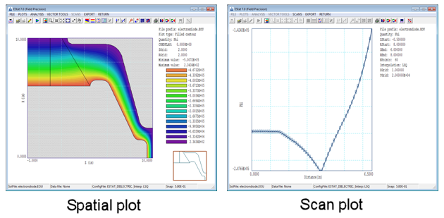
Figure 1. Spatial versus scan plots in TriComp programs.
The simplest application of saved views is to restore a complex plot when you reload the solution at a later time. We have included several features in our implementation to enable a higher level of data analysis:
- A saved view works even if a completely different solution than one use to create the view in loaded. In fact, views can be reloaded even if the user is running a different TriComp program. The current program analyzes the parameters and uses only ones that are relevant. For example, if a view-boundary or scan point is outside the current solution volume, the point is moved to the boundary. If a plot quantity is undefined, the first valid quantity is used.
- A free-form parser is employed when a view is loaded. Therefore, a file need not contain a complete set of parameters. Changes are made only to the quantities listed in the file.
- Users can modify entries in the view file, either directly with an editor or via a Perl or Python script. You can include comments, change parameter values or remove parameter lines.
Another important feature is related to the fact that analysis functions of all TriComp postprocessors may be controlled by a text script. We have added the following script command:
PLOT FSaveView FOutput Nx Ny
PLOT (DiodeRegion VIEW001 800 600)
The string FSaveView is the prefix of a saved view file. The string FOutput is the prefix of a plot file in BMP format. The integer parameters give the image resolution in pixels. In response to the command, the program loads the saved view file, applies the parameters to create a plot for the currently-loaded solution and saves it as a graphics file.
Here are some possible scenarios:
- You have a set of electric field solutions with different applied voltage and possibly different boundaries and you want to check electric field levels in a critical region (e.g., an electron source). Use the Zoom command to create the desired plot and save a view file. Remove all information lines except the view boundaries and load the view when you load a different solution.
- You have a set of magnetic field solutions and want precision plots of field lines passing through specific points. Add a field line interactively in PerMag and save a template view file. Then edit the view file to remove unnecessary information, change the number of field lines and add coordinates for the desired points.
- You want to create a large set of radial temperature scans moving along the axis of a probe assembly. In TDiff, create a template view file for one scan. Write a Python or Perl script with a loop of axial positions that modifies the axial scan coordinates in the view file and then runs TDiff in the analysis mode. The set of BMP files could then be stitched into an AVI movie with our Cecil_B utility.
- A sequence of annotated view files could be employed in a training session or educational demonstration.
- You want to show how the levels of magnetic flux induction change with changing coil currents, preserving magnitude scaling in the plots. After creating a set of solutions, load one of them adjust the view, plot style and plot quantity. Turn off autoscaling, specify values for BMin and BMax and then save a view file. Load the view for the other solutions.
LINKS
