Linear quadrupoles are widely used for ion mass spectrometry. They can separate ions by the ratio of mass number to charge number (M/Z) without a magnetic field, leading to compact, light and inexpensive systems. An assembly consists of a source of low-energy ions that enter an extended electrostatic quadrupole. The voltage applied to the lens has both DC and AC components. The orbits of most ions are unstable. Depending on the choice of voltages and RF frequency, only ions within a small range of M/Z have stable orbits and pass to a downstream detector. This report demonstrates the application of the three-dimensional OmniTrak code to characterize quadrupole mass analyzers.
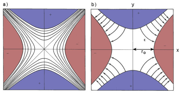
Figure 1. Cross-section of an electrostatic quadrupole. a}) Lines of constant potential. b}) Electric field lines.
Assume the quadrupole has ideal hyperbolic electrodes with an electrode-tip radius r0 (i.e., the distance from the axis to the closest point on an electrode). The beam propagates in the z direction. Figure 1 shows a cross section of the geometry in the x-y plane. The voltage applied to the top and bottom electrodes has the form of Eq. 1 where U is the DC component and V is the magnitude of the RF voltage with angular frequency O. Voltages with opposite polarity are applied to the y and x electrodes.
The electrostatic potential in the gap has the form of Eq. 2. The y component of electric field is given by Eq. 3. Equation 4 describes ion motion in the y direction. With the introduction of the dimensionless variables of Eqs. 5, 6 and 7, the equation of motion takes the form of Eq. 8. Motion in the x direction is described by Eq. 9.
Equations 8 and 9 must be solved numerically. There are regions in (a,q) space where ion motion in x or y may be stable or unstable. Here, the term stable implies that the trajectories are bounded oscillations. In unstable regions, the displacement increases exponentially so that in a short time ions strike the electrodes. In particular, ions have stable trajectories in both the x and y directions within the shaded region shown in Figure 2. (Note that there is also a symmetric stability region below the q axis. Changing a to -a simply exchanges the roles of x and y).
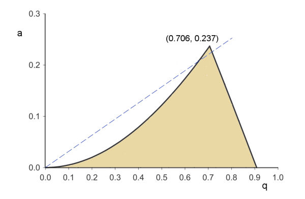
Figure 2. Region of a-q space with stable motion in both x and y.
For reference, note that the ratio of the parameters is proportional to the DC voltage component divided by the AC component (Eq. 10). A fixed ratio corresponds to a straight line in (q,a) space like the dashed line in Fig. 2. Motion along the line starting at the origin is equivalent to raising the magnitude of U and V while keeping a constant ration. For a section of the scan, the curve in Fig. 2 passes through the stability region. The tip of the stability region has the coordinates q = 0.706 and a = 0.237.
The operation of the quadrupole as a mass filter is clear if we plot regions of stability in terms of voltage values U and V rather than the dimensionless parameters a and q. Figure 3 shows stability regions for two values of M/Z. The M/Z value for the green shaded region is half that of the tan region. The working line follows a fixed voltage ratio, U/V < (0.237)/(2 × 0.706). Note that as the magnitude of the applied voltages increases, the working line first passes through the green stability zone and then through the tan zone. A plot of the detector response versus a scan of voltage magnitude will show two peaks corresponding to the two values of (M/Z). Higher voltages correspond to higher mass-to-charge ratios. Absolute values of (M/Z) may be inferred from known values of the voltage, quadrupole geometry and RF frequency. Note that the ratio U/V = 0.168. gives ideal resolution but no throughput. Lowering the DC voltage allows more particles to pass to the detector at the expense of reduced mass resolution. With no DC offset (U = 0), all ions pass through the quadrupole.
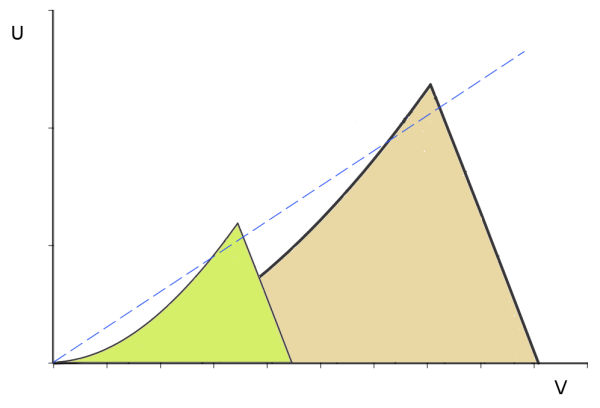
Figure 3. Stability regions and a working line for ion transport as a function of the applied voltages U and V. The shaded regions show the stability zone for two ion species. The green region has a mass to charge ratio (M/Z) equal to half that of the tan region.
We now have the theoretical resources to design a practical system. Take the quadrupole length as L = 15.0 cm. Fabricating hyperbolic electrodes is expensive, so we'll use stock electrodes with a circular cross section to approximate the field. The choice is acceptable as long as the ions are confined close to the axis. The electrode diameter is d = 1.0 cm. The electrodes are displaced 0.9 cm from the propagation axis, giving the minimum distance from the axis to an electrode of rc = 0.4 cm. We can identify two questions that can be answered by a 3D code:
- How does the choice of rc versus d affect the linearity of electric fields near the axis?
- What is the value of ro for equivalent hyperbolic electrodes? In other words, if we used hyperbolic instead of circular electrodes with a given voltage, what choice of ro would give the same electric field variation near the axis?
We'll concentrate on the second issue, calculating the electric field with HiPhi. The quadrupole assembly is centered in a solution volume that covers the range -3.0 cm = x,y = 3.0 cm and 0.0 cm = z = 20.0 cm. The wall of the solution volume is grounded. The element size in the quadrupole region is 0.05 cm. Figure 4 shows the resulting mesh.
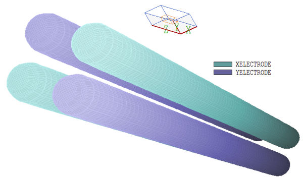
Figure 4. Conformal representation of the quadrupole electrodes.
I used normalized voltages of +1.0 V on the y electrodes and -1.0 V on the x electrodes in the electrostatic solution. Figure 5 shows calculated values of Ex in a scan through the axis along x at the quadrupole center. Over the range -0.2 cm = x = 0.2 cm, the field varied linearly with x to within 0.01%. The calculated dependence is Ex(x) = (1.255 × 10^5)x V/m. A comparison with Eq. 3 for hyperbolic electrodes implies the relationship of Eq. 11. The equivalent hyperbolic pole tip distance is 0.3993 cm, quite close to the physical distance rc = 0.4000 cm. My initial guess of rc = 0.4 d turned out to give excellent results.
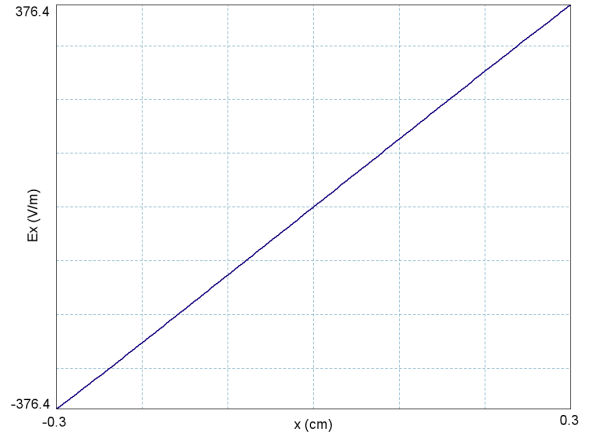
Figure 5. Scan of Ex(x) at position y = 0.0 cm, z = 10.0 cm for normalized electrode voltage magnitude of 1.0 V.
The electrostatic solution was used as a basis for OmniTrak calculations of ion trajectories. I concentrated on singly-charged carbon ions (M = 12, Z = 1) with an initial kinetic energy of 40 eV. The drift velocity was 2.5 ? 10^4 m/s, so the transit time through the spectrometer was about 6 ?s. There should be several RF periods over the transit time to ensure that ions experience an average focusing force. I picked f = 2.5 MHz, corresponding to O = 1.571 × 10^7 1/s. A time step choice of ?t = 10.0 ns gave an acceptable value of 40 integration steps per RF period. I picked the PList command to initiate ion trajectories near the z = 0.0 cm boundary with velocity directed along z. To sample positions in x-y space, I used a spreadsheet to create a circular distribution of 36 particles at radius 0.1 cm. (There was no point in representing an on-axis particle. It would traverse the system with no transverse motion in all circumstances). Equations 6 and 7 can be used to find the U and V values for a working line that passes through the tip of the stability region (Fig. 2). Taking a = 0.237, q = 0.706 and substituting values for the quadrupole leads to the Eqs. 12 and 13.
The values for carbon ions are U = 14.65 V and V = 87.28 V. The value of U must be lower to observe transmitted ions.
The full OmniTrak input script is listed at the end of the report. The critical commands to represent the RF quadrupole are:
EFIELD3D: QuadAnalyzer.HOU 0.9875
MODFUNC E > 14.0 + 87.28*sin(1.571E7*t)
The first command loads the normalized electric field. The adjustment factor (ß= 0.9875) determines the voltage magnitude and hence the position along the working line. We can make small changes to study the transmission width of an ion type, or large changes to study a different type. For example, the adjustment factor for singly-ionized iron is about ß = (56/12) = 4.67. The ModFunc command serves two functions:
- Add a time variation of fields during the ion transit.
- Set the slope of the working line (i.e., determine the acceptance of the system).
With regard to the first function, all values of potential in the electrostatic solution are multiplied by the current value of the algebraic function. This process is valid when the propagation distance of an electromagnetic signal over an RF period is much larger than the system.
My procedure was to set a value of U less than 14.65 V in the ModFunc command and then to do a series of runs with varying ß to change the total voltage level. Figure 6 shows the results for U = 12.0 V and 14.0 V. As expected, the peak signal occurred near the tip of the stability region and a lower value of U gave an increased transmission width. Figure 7 shows the effect of small changes of ß on ion trajectories.
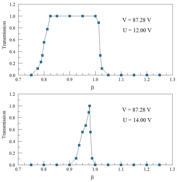
Figure 6. Particle transmission factor as a function of the relative voltage magnitude and U.
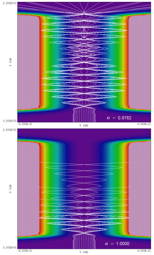
Figure 7. Projected carbon ion trajectories in the z-y plane for V = 87.28 V and U = 14.0 V. A small change in the applied voltage magnitude causes transmission to drop from 100% to 0%. Note that the y scale has been expanded for clarity.
Finally, note that the calculation procedure can be automated for extended data analyses in the background. For example, to make a scan in voltage magnitude, the EField3D command could be changed to
EFIELD3D: QuadAnalyzer.HOU %1
where %1 represents a command line parameter. Multiple OmniTrak calculations could be controlled with a batch file with a form like this:
REM Xenos batch file, Field Precision
REM
START /B /WAIT C:\fieldp_pro\xenos/omnitrak.exe QuadAnalyzer 0.75
RENAME QUADANALYZER.PRT QuadAnalyzer01.PRT
REM
START /B /WAIT C:\fieldp_pro\xenos/omnitrak.exe QuadAnalyzer 0.80
RENAME QUADANALYZER.PRT QuadAnalyzer02.PRT
REM
START /B /WAIT C:\fieldp_pro\xenos/omnitrak.exe QuadAnalyzer 0.85
RENAME QUADANALYZER.PRT QuadAnalyzer03.PRT
REM
START /B /WAIT C:\fieldp_pro\xenos/omnitrak.exe QuadAnalyzer 0.90
RENAME QUADANALYZER.PRT QuadAnalyzer04.PRT
...
The end result is a set of particle files that may be analyzed with a text editor or a user script to find the fraction of particles that reach z = 20.0 cm.
Example: OmniTrak input script
FIELDS
  EFIELD3D: QuadAnalyzer.HOU 0.9782
  DUNIT:   1.0000E+02
  MODFUNC E > 14.0 + 87.28*sin(1.571E7*t)
END
PARTICLES TRACK
  DT  1.0E-8
  PLIST
    12.0  1.0  40.0  0.0996   0.0087 0.01 0.00 0.00 1.00
    12.0  1.0  40.0  0.0966   0.0259 0.01 0.00 0.00 1.00
    12.0  1.0  40.0  0.0906   0.0423 0.01 0.00 0.00 1.00
    12.0  1.0  40.0  0.0819   0.0574 0.01 0.00 0.00 1.00
    12.0  1.0  40.0  0.0707   0.0707 0.01 0.00 0.00 1.00
    12.0  1.0  40.0  0.0574   0.0819 0.01 0.00 0.00 1.00
    ...
    12.0  1.0  40.0  0.0574  -0.0819 0.01 0.00 0.00 1.00
    12.0  1.0  40.0  0.0707  -0.0707 0.01 0.00 0.00 1.00
    12.0  1.0  40.0  0.0819  -0.0574 0.01 0.00 0.00 1.00
    12.0  1.0  40.0  0.0906  -0.0423 0.01 0.00 0.00 1.00
    12.0  1.0  40.0  0.0966  -0.0259 0.01 0.00 0.00 1.00
    12.0  1.0  40.0  0.0996  -0.0087 0.01 0.00 0.00 1.00
  END
END
DIAGNOSTICS
  PARTFILE: QuadAnalyzer
END
ENDFILE
Download a PDF version of this report: quadmassanalyzer.pdf
LINKS
