OmniTrak is our software package for charged-particle guns and beam dynamics. The solution program can read output files from HiPhi and Magnum for 3D electric and magnetic field information. These complex files record values of potential on conformal meshes. Tables are another option for field information. Tables record [Ex,Ey,Ez] or [Bx,By,Bz] on a regular box mesh. Table files are easy to create and facilitate import of field information from other programs. Sometimes, it is useful to use an intermediate table instead of directly reading information from HiPhi and Magnum. In this case, the user uses the MATRIX command in PhiView or MagView to convert the values of potential on the conformal mesh to a table of electric field or magnetic flux density values. This reduces the amount of work performed by OmniTrak and can speed up many calculations.
A user recently suggested another application of tables that is helpful when the fields of a magnetic transport element can be expressed as a linear superposition of the fields produced by different control coils. For example, it may be useful to model the performance of a magnetic scanning system by calculating orbits for several values of current in the the X and Y drive coils. A quick way to do the calculation would be to prepare tables for the fields of the X and Y drive coils with a normalized current, and then to load a superposition of the fields into OmniTrak with different scaling factors. The process could be controlled by a batch file for a parameter search.
Recently, we make changes to OmniTrak to enable this procedure. The command to load a table has the form
BTable3D COIL01.MTX 1.5
where COIL01.MTX is the name of the table in the working directory and 1.5 represents an optional scaling factor. The factor multiples values of [Bx,By,Bz] — the number may be positive or negative. In the past, a second BTable3D command would simply cause the previous table to be overwritten. In the current version of OmniTrak, multiple BTable3D statements result in a superposition of values. There is no limit to number of commands — here is an example with two:
BTable3D COIL01.MTX 1.5
BTable3D COIL02.MTX 2.0
OmniTrak reads the first table in the normal way with scaling factor 1.5. When the second command is encountered, the program opens the file and checks that the map parameters (IMax, JMax, KMax, Xmin, Xmax, Ymin,...) are identical. If so, OmniTrak reads the second table and adds values of {Bx,By,Bz] to those already in memory with the scaling factor 2.0. In summary:
- There is no limit to the number of BTable3D commands.
- Multiple maps must use the same mesh.
- BTable3D commands may appear in any order in the FIELDS section of the OmniTrak script.
- Shifts and rotations are applied after all tables have been superimposed.
- The user must ensure that the superposition is physically valid.
- The ETable3D command has also been extended.
Figure 1 shows data from a test example: two identical shielded solenoid lenses at different positions along the z axis. The blue squares represent the tabular field of the first coil and the red squares show the field of the second downstream coil. The line is the total field calculated with the OmniTrak BSCAN command resulting from the command set listed above. The following parameters were used in the Magview MATRIX command to create the tables: IMax = 21, XMin: -10.0, XMax = 10.0, JMax = 21, YMin = -10.0, YMax = 10.0, KMax = 240, Zmin: -12.0 and ZMax = 12.0.
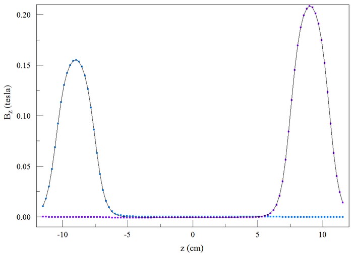
Figure 1. Test case - superposition of two solenoid lenses.
LINKS
