The term End-to-end simulation has a mystical power in calculations of charged-particle devices. In the end-to-end simulation, the user inserts starting conditions and the code handles everything thereafter, presumably with all the physics included. The user retires and finds, upon returning, that the code has passed the answer. The allure of the end-to-end simulation lies in two assumptions:
- Any contribution from the user will mess things up.
- Being expensive, the codes must be right.
In reality, end-to-end simulations are often inefficient and inaccurate. Furthermore, they often impede user learning experiences.
In the TriComp and AMaze programs, I have used multistage techniques wherever possible. Division of a calculation into parts often saves considerable time and even offers improved accuracy. Nonetheless, I have found users are often nervous about planning multistage strategies in a program like Trak because they are not sure they are doing everything right. Hopefully, this article will help. In it, I will step through a two stage Trak calculation, emphasizing the decisions I made along the way.
Figure 1 shows the global geometry. The components of a 120 kV, 2 A electron gun are on the left-hand side: focusing electrode (violet), cathode and emission surface (blue) and grounded anode (tan). The gun was designed to produce a narrow focus at the exit of the anode aperture. The beam then transversed a grounded vacuum section with 2.0 cm radius to a target at 20 cm distance. A solenoid lens was used to focus the beam at the target.
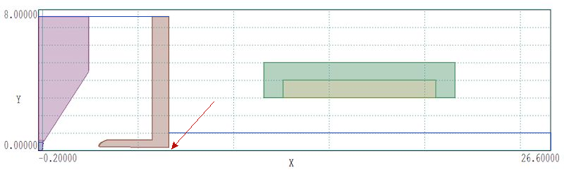
Figure 1. Global geometry: electron gun and focusing solenoid.
There are two tasks:
- Vary the gun-electrode geometries: a) to achieve the target current and b) to ensure a small radius beam at the anode aperture exit (red arrow).
- Adjust the lens current to produce a focus at the target.
Although it is easy to set up a Trak solution that handles the full system from cathode to target, it is more efficient to design the gun and then to address the focusing system. Figure 2 shows the final gun solution, defined by the input files multistage01.min, multistage01.ein and multistage01.tin (a link to a zip file with all input files appears at the end). A magnetic-field solution was not included because the flux produced by the shielded solenoid lens was less than the earth's field in the gun region. The self-consistent gun current was 1.93 A. The beam envelope radius at the exit was about 0.45 mm.
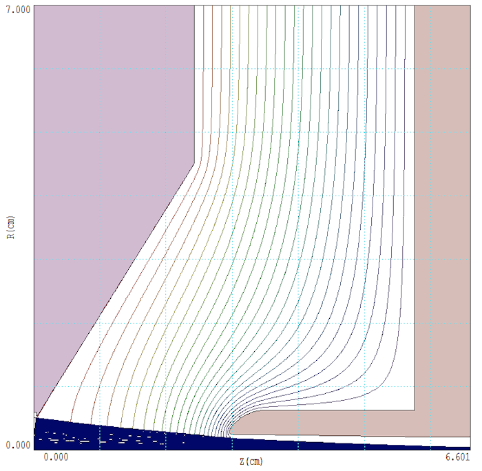
Figure 2. Electron gun solution (multistage01).
Here's listing of multistage01.tin:
FIELDS
  EFile = multistage01.eou
  DUnit = 100.0
END
PARTICLES RELBEAM
  NCycle = 25
  Emit(5) 0.0 -1.0 0.0100 2 1.0E8 0.1
  Avg = 0.25
  Dt = 1.0E-12
END
DIAGNOSTICS
  Partlist Cylin
  PartFile Multistage01P
  EDump = Multistage01P
  BBDump = Multistage01P
END
ENDFILE
The RelBeam mode was used because of the high gun voltage (120 kV). The Emit statement demonstrates generation of a beam with a transverse temperature distribution. The right-hand boundary had two features to enabled coupling to a second solution for the lens region:
- The location was set a 6.601 cm rather than 6.600 cm.
- The Neumann condition applies over the exit aperture.
The slight shift of the boundary ensured that the extrapolated axial positions of all particles in the output PRT file were?? 6.60 cm. The idea was to avoid Not in solution region errors when starting the electrons in the second solution. The Neumann condition ensured that equipotential lines were normal to the boundary over the aperture and that the beam-generated potential was not shorted. A conducting foil over the aperture (Dirichlet condition) would give virtual electron focusing.
The second solution for the lens region with both magnetic and beam-generated electric fields had input files multistage02.min, multistageb.min, multistage02.ein, multistageb.pin and multistage02.tin. The magnetic field solution (multistageb.min, multistageb.pin) covered the region 6.6 cm?? z?? 26.6 cm, 0.0 cm?? r?? 8.0 cm. The initial value of the drive current was 1000 A-turn. Anticipated field levels were well below the saturation value of the magnet-steel flux core, so a fixed value of ?r = 500 was used for the magnetic permeability. The peak field on axis was 142 G. An electrostatic mesh to calculate beam-generated fields covered the region 6.6 cm ≤ z ≤ 26.6 cm, 0.0 cm ≤ r ≤ 2.0 cm (multistage02.min, multistage02.ein). There was no applied electric field. The vacuum region was surrounded by grounded walls except for a Neumann condition applied over the entrance aperture. The Neumann boundaries in the first and second solution ensured an approximate match between the two electrostatic solutions (i.e., same variation of beam-generated potential at the aperture).
The Trak file multistage02.tin had the content:
FIELDS
  EFile = multistage02.eou
  BFile = multistageb.pou? 4.1
  DUnit = 100.0
END
PARTICLES SCHARGE
  PFile multistage01P
  NCycle = 15
  Avg = 0.25
  Dt = 2.0E-12
  RelMode
END
DIAGNOSTICS
  Partlist Cylin
  PartFile Multistage02P
  EDump = Multistage02P
END
ENDFILE
Both electric and magnetic fields were included in the calculation. Note the multiplication factor for the magnetic solution. Because the solution is linear (fixed μr), we can check different field strengths simply by multiplying all values of the vector potential by a constant. Because there were no applied axial electric fields, the solution could be performed in the SCharge mode with the RelMode option. In this case, the code calculated beam-generated electric fields and reduced the force by 1/γ^2 (the theory underlying the RelMode is reviewed in the Trak manual). This approach is quicker and more accurate than assigning beam current elements to a mesh and calculating B? directly. Because of the close balance between electric and magnetic forces for relativistic electrons, small errors in the two calculations have a relatively larger effect. Entrance particle parameters were set from the PRT output file from the first calculation (multistage01p.prt). The electrons started close to the left-hand boundary.
Figure 3 shows the beam solution with no magnetic field (field multiplication factor set equal to 0.0). Beam-generated forces caused an expansion. The peak beam-generated potential at the entrance aperture was about -800 V. The calculation run time was a few seconds, so it was easy to optimize the lens by trial and error, changing the magnetic field multiplication factor to approach to the best solution. Figure 4 shows the final result, with a multiplication factor of 4.1 (4200 A-turn, peak field of 582 tesla). Note that if we hadn't split the solution, it would be necessary to recalculate the gun solution for each iteration, a needless activity.
Download the input files: multistage.zip.
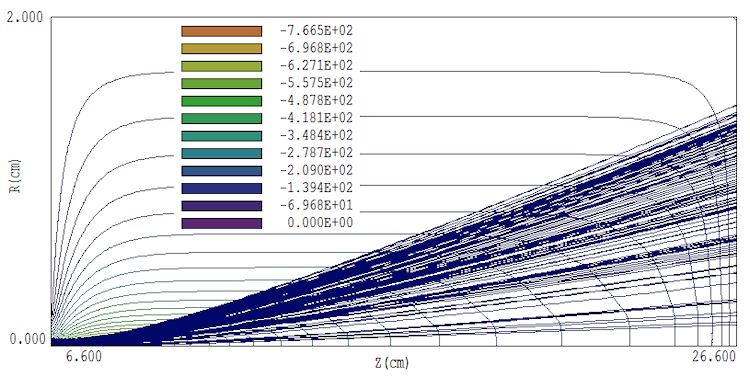
Figure 3. Beam expansion with no lens field.
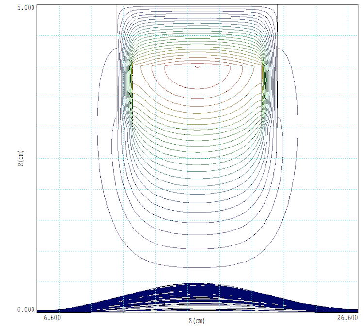
Figure 4. Solution with 4100 A-turn, expanded radial scale.
LINKS
