Aether can transfer three-dimensional power-density distributions calculated in the RF mode to HeatWave for thermal simulations. A user suggested an application — heating of dielectric objects in a microwave resonator. We carried out detailed calculations for this application to test the new code features and to confirm the existing capabilities of the two-dimensional codes WaveSim and TDiff. This article illustrates how to set up coupled RF/thermal solutions and how to ensure the validity of results. The input files are available for download at the end of the article.
Figure 1 shows the geometry for the benchmark solution. The system has cylindrical symmetry so we could make comparisons between the two- and three-dimensional results. A mode of type TM010 was generated in the cavity of radius Rc = 15.0 cm and length D = 12.0 cm. The theoretical frequency for the empty cavity is 765.54 MHz. The dielectric object had radius Ro = 5.0 cm and length Do = 6.0 cm. The electromagnetic mode was generated by a current density source in the shape of a thin plate that acted as a capacitive driver.
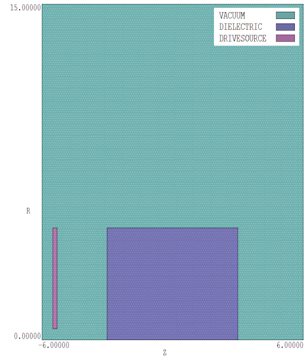
Figure 1: Geometry of the test calculation, dimensions in cm, cylindrical symmetry.
Before discussing the WaveSim/TDiff solutions, it is useful to review what we mean by heating in a resonant cavity. The assumption is that the power absorbed by the dielectric object does not significantly distort the resonant electric and magnetic fields. In other words, the total system has a high Q value. In this case, the field distribution is almost independent of the geometry of the driver; therefore, it is not necessary to make a detailed model of the power coupler (e.g., coupling loop or waveguide), an impossible task with a two-dimensional code. The implication is that we must exercise care in choosing the electrical conductivity of the dielectric.
The element size in the Mesh input file ( HeatingDemo2D.MIN) was relatively small for high resolution, 1.0 mm. A uniform element size was used throughout the solution volume to avoid the possibility of instabilities in the TDiff calculation. In a WaveSim H-type solution, the boundaries of the solution volume act as ideal conducting walls, so there is no need to define wall elements. The WaveSim input file HeatingDemo2D.WIN has the content:
Mesh HeatingDemo2D
Geometry = Cylin
DUnit = 100.0
Solution = H
Mode = Search
* Range = (700.0E6 800.0E6)
Range = (600.0E6 650.0E6)
FStep = 15
Tolerance = 1.0E-6
Probe = (0.0, 14.0)
* Vacuum
 Mu(1) = 1.0
 Epsi(1) = 1.0
* Dielectric
 Mu(2) = 1.0
* Empty cavity
* Epsi(2) = 1.0
* Ideal dielectric
* Epsi(2) = 12.0
* Dielectric absorber
 Epsi(2) = 12.0,1.2E-5
* Drive source
 Mu(3) = 1.0
 Epsi(3) = 1.0
 Source(3) = (1.0, 0.0, 0.0)
ENDFILE
The source region has current density pointing in the z direction. In a resonant solution, the amplitude of the source and resulting fields is arbitrary. We can normalize the fields to achieve desired power levels. There are three definitions for the dielectric controlled by comment-line symbols: 1) ideal vacuum, 2) ideal dielectric with relative dielectric constant εr = 12.0 and an absorbing dielectric with εr = 12.0 and εr" = 12.0 × 10⁻⁶. With no dielectric, WaveSim gives a resonant frequency of 764.9 MHz. The frequency drops to 626.33 MHz with the addition of the dielectric. Figure 2 shows lines of applied electric field.
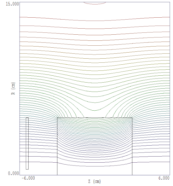
Figure 2: Solution with dielectric, lines of applied electric field.
In WaveSim, imperfect dielectrics are defined by adding an imaginary part of the relative dielectic constant, εr". Power losses may result from conductivity or a phase lag in the dielectric response. In the case of resistivity losses, the conductivity and imaginary part of the dielectric constant are related by
σ = 2πf ε0 εr"
where f is the mode frequency. The loss power density is related to the imaginary part of the dielectric constant and local electric field by
<p> = 2πf ε0 εr" |E2|/2.
The time-averaged electric field energy density is
ue = ε0 εr |E2|/4.
Combining the equations, the time-averaged power loss can be written in terms of the time-average electric field energy density:
= 4 π f (εr"/εr) ue.
The implication is that the system will have high Q if εr" ≪ εr. Note in the WaveSim input file that that the ratio is 10-6, so the condition of high Q is well satisfied.
As expected, dielectric losses did not significantly affect the resonant frequency (f = 626.33 MHz). By chance, the field and power levels in the WaveSim solution were in a range of interest for a thermal calculation, so it was not necessary to re-normalize the field. The electric field magnitude on axis at z = 0.0 cm was 4.641 MV/m and the power density was 4.503 MW/m3. The global electric field energy in the dielectric region was 0.1327 J and the absorbed power loss was 1.04452 kW, in agreement with predictions.
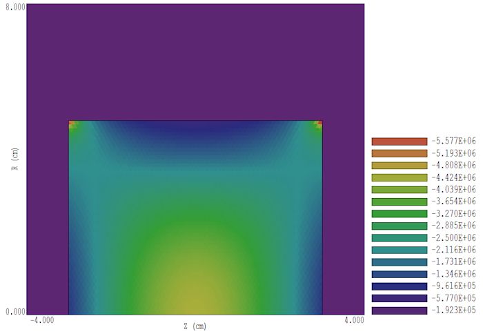
Figure 3: Absorbed power density inside the dielectric in W/m3.
The next step was to use the WaveSim output as a source in a dynamic TDiff calculation. The TDiff input script had the content:
* ---- CONTROL ----
Mesh = heating_demo2D
Mode = TVar
Geometry = Cylin
DUnit = 1.0000E+02
TMax = 1.1000E+01
DtMin = 1.0000E-03
DtMax = 2.0000E-02
Safety = 5.0
SourceFile heating_demo2D.wou
* ---- REGIONS ----
* Region 1: VACUUM
 Cond(1) = 1.0000E-03
 Cp(1) = 1.0000E+00
 Dens(1) = 1.0000E+00
* Region 2: DIELECTRIC
 Cond(2) = 1.0000E-01
* Cond(2) = 1.0000E+01
 Cp(2) = 1.2000E+03
 Dens(2) = 1.3000E+03
* Region 3: DRIVESOURCE
 Cond(3) = 1.0000E-03
 Cp(3) = 1.0000E+00
 Dens(3) = 1.0000E+00
* Region 4: AXIS
 Cond(4) = 1.0000E-03
 Cp(4) = 1.0000E+00
 Dens(4) = 1.0000E+00
* ---- DIAGNOSTICS ----
DTime = 1.0000E+01

EndFile
The thermal calculation was performed on the same mesh as the WaveSim solution. The vacuum regions were assigned a low thermal conductivity, specific heat and mass so they had negligible effect on the thermal balance in the dielectric. Temperature distributions in vacuum were ignored. The line region on axis (Region 4) necessary for the WaveSim solution played no part in the TDiff calculation. It was assigned the material properties of vacuum to ensure that the nodes were treated as variable temperature.
The parameters for the dielectric were chosen arbitrarily to give a valid thermal solution: Cp = 1200 J/kg-oC and ρ = 1300 kg/m3. In the first run, the conductivity was set low (k = 0.1 W/m2-oC) to make a comparison with theory. For average power density <p>, the predicted temperature rise with no thermal conductivity is
ΔT = (<p> /ρCp) Δt.
Using the WaveSim power density at the midpoint on axis,the predicted maximum temperature at the end of the 10 second run was 29.75oC.
The top of Fig. 4 shows the temperature distribution in the dielectric calculated by TDiff at 10.0 s. The temperature at the reference point (z = 0.0 cm, r = 0.0 cm) was 28.86 oC. In a second run, the conductivity was set to a high value, k = 10.0 W/m2-oC. In this case, the temperature profile was more diffuse and the value at the reference point was 25.60 oC.
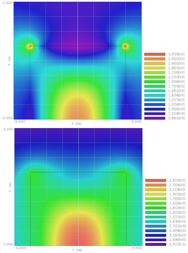
Figure 4: Temperature distributions calculated by TDiff with different dielectric thermal conductivities. Top: k = 0.1 W/m-degC. Bottom: Top: k = 10.0 W/m-degC.
The same calculation was performed with Aether and HeatWave using the capability to share power-density profiles. The solution used the same geometry and material properties as the two-dimensional calculation. In the MetaMesh input file HeatingDemo3D.MIN, an element width of 5.0 mm was used for a short run time. Therefore, we would not expect to resolve fine details like the field enhancement on the sharp edges of the dielectric in Fig. 2. Figure 5 shows a cutaway view of one quarter of the mesh. Note that a regular mesh is required for an Aether calculation. Despite the box elements and the relatively coarse zoning, both the microwave and thermal solutions were close to the two-dimensional results. In contrast to WaveSim, in Aether an outer region of elements with the properties of a perfect conductor is necessary to define the walls of the cylindrical cavity. The inner surface of this region is shown in blue in Fig. 5. The dielectric (violet) and drive region (red) had the same shape as those in the two-dimensional calculation.
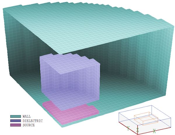
Figure 5: Mesh geometry for the Aether and HeatWave calculations showing one-quarter of the solution volume.
Another difference in Aether is that the solution must be performed in two parts: 1) identification of the resonant frequency and 2) calculation of the field distribution at that frequency. Here is the Aether input file for the resonance solution:
* ---- CONTROL ----
 Mode = RES
 Mesh = Heating_Demo3D
 DUnit = 100.0
 Freq 0.60E9 0.30E9
 Source 3 0.0 0.0 1.0
 Parallel 6
 * ---- REGION PROPERTIES ----
 Metal(1)
 Vacuum(2)
 Epsi(3) 12
 Sigma(3) 4.178.8E-7
 Vacuum(4)
 * ---- DIAGNOSTICS ----
 Probe = 14.500 0.000 0.000 Hy
EndFile
The calculated frequencies were 766.7 MHz with no dielectric and 626.12 MHz with the dielectric (both ideal and conducting). The agreement with WaveSim was better than 0.25%. Another difference is that Aether requires specification of the conductivity rather than imaginary part of the dielectric constant. The value ? = 4.178.8 ?10?7 S/m was determined from Eq. 2 with f = 626.12 MHz.
The Aether input script for the second solution had the control entries
Mode = RF
Freq   6.261167E+08
NPeriod  15  3  10
An RF mode calculation differs from a RES mode calculation in two ways: 1) it is performed at specific drive frequency and 2) Aether creates a data file of the field and power-deposition distributions. This data may be transferred to HeatWave. The parameters in the NPeriod command have the following meaning. Run the time-domain solution for 15 RF periods. The current in the drive region should start smoothly over 3 periods and stop after 10 periods to let the fields come to equilibrium. At the end of the run, Aether determines the amplitude and phase of field quantities to find complex number values for the output file.
The amplitude of the drive current was set to the arbitrary value Jz = 1.0 A/m2. Therefore, it was necessary to normalize the field for a comparison with the WaveSim results. The Aerial postprocessor showed that the electric field at the reference point was Ez = 4.2384 V/m, compared to the WaveSim result of 4.641 ?106 V/m. A factor of 1.0844 ?106 was entered in the Analysis/Normalize command of Aerial and the result was saved as the file HeatingDemo3DNorm.aou.
The HeatWave input file had the content:
* ---- CONTROL ----
Mesh = heating_demo3D
Mode = Dynamic
DUnit =   1.000000E+02
TMax =   1.100000E+01
DtMin =   1.000000E-03
DtMax =   5.000000E-03
SourceFile HeatingDemo3DNorm.aou
* ---- MATERIAL PROPERTIES ----
* Material 1
Cond(1) =   1.000000E-03
Cp(1) =   1.000000E+00
Dens(1) =   1.000000E+00
* Material 2
Cond(2) =   1.000000E-03
Cp(2) =   1.000000E+00
Dens(2) =   1.000000E+00
* Material 3
* Cond(3) =   1.000000E+01
Cond(3) =   1.000000E-01
Cp(3) =   1.200000E+03
Dens(3) =   1.300000E+03
* Material 4
Cond(4) =   1.000000E-03
Cp(4) =   1.000000E+00
Dens(4) =   1.000000E+00
* ---- REGION ASSIGNMENTS ----
* Region 1: WALL
Region(1) =   1
* Region 2: VACUUM
Region(2) =   2
* Region 3: DIELECTRIC
Region(3) =   3
* Region 4: SOURCE
Region(4) =   4
* ---- DIAGNOSTICS ----
DTime =   1.000000E+01
EndFile
The new capability to import Aether power profiles appears in the command SourceFile HeatingDemo3DNorm.aou. Figure shows the resulting temperature distribution in the dielectric at 10 seconds for thermal conductivity k = 0.1 W/m2-oC. The temperature at the reference point was 28.33 oC, within 2% of the TDiff prediction. At high conductivity (k = 10.0 W/m2-oC) the value was 25.17 oC, comparable to the TDiff result of 25.60 oC.
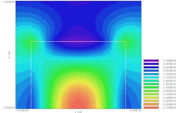
Figure 6: Temperature distribution calculated by HeatWave for a thermal conductivity k = 0.1 W/m-degC.
Use this link to download a PDF report on this work:? Microwave heating simulations. Use this link to download the program input files: HeatingDemoFiles.zip.
LINKS
