A common task in computer calculations in collective physics is the generation of input particles with a desired probability distribution in energy, angle or position. This article discusses some easy methods to accomplish the task using a software module to manipulate tabular functions. As an example, we'll consider creating a Maxwell-Boltzmann distribution in kinetic energy U.
As a preliminary, let's review some probability theory. A distribution of particles with respect to a quantity like energy is represented as a probability density. The probability density p(x) is defined as follows: the probability of observing a value of x in the interval x0 -?x/2 to?x0 +?x/2 is approximately given by Eq.(1).
The marginal probability is given by Eq.(2). Figure 1 shows the relationship of the two functions. If p(x) is a normalized function, then the marginal probability has the range 0.0 ≤ P(x) ≤ 1.0. The function gives the probability of observing a value of x between x(min) and a specified maximum value. The marginal probability has another interpretation illustrated by the shaded region of Fig. 1. The interval along the P(x) axis represents a fraction of the particles (5% in the figure). These particles are distributed along an interval of the x axis with a length inversely proportional to the slope of P(x), or 1/p(x). The particle density along x is low where p(x) is small and high where p(x) is large. In other words, a uniform distribution along the vertical axis maps into a non-uniform distribution along the horizontal axis with density proportional to p(x).
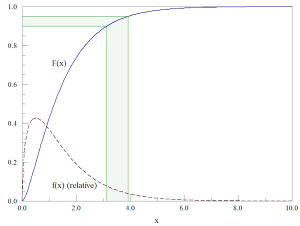
Figure 1. Relationship between the probability density and the marginal probability for a Maxwell-Boltzmann energy distribution.
The observation suggests the following procedure to create N model particles with probability density p(x). First, find N uniformly-distributed values of the variable ζ in the interval 0.0 ≤ ζ ≤ 1.0. Second, use the inverse of the marginal probability function to create N particles with quantity values given by Eq.(3).
There are potential problems applying the procedure in a code:
- The probability density p(x) may not be normalized or integrable.
- There may be no closed form to express the inverse of the marginal probability.
- The probability density may extend to infinity.
All three items apply to the Maxwell-Boltzmann distribution. The first two issues can be resolved by using a numerical approach that does not involve closed-form expressions. To resolve the third issue, it is necessary to truncate distributions at a finite value.
Tabular functions constitute a useful tool for generating particle distributions. My introduction to the concept was in the program SciMath developed by Robert Kares. It was remarkably easy-to-use software from the DOS era that was unfortunately eclipsed by programs like Mathematica and MathCad. A tabular function in SciMath was a set of discrete values of an independent variable xi and a dependent variable yi(xi). By using a variety of numerical techniques, the program made interpolations and calculated integrals and derivatives. To the user, tabular functions could be employed as though they were continuous functions. I wrote a module to define tabular function variables and to perform operations almost two decades ago.
Let's see how to apply tabular functions to create a Maxwell-Boltzmann energy distribution. The probability distribution of kinetic energy scales as Eq.(4), where x = U/kT for the temperature T in °K. My general approach is to do one-time setup calculations with a spreadsheet and to incorporate repetitive operations in the code. The first column in my spreadsheet contained 200 values of x over the range 0.0 ≤ x ≤ 10.0. The second column contained non-normalized values of p(x) from Eq.(4). The third column was the definite integral of p(x) using the trapezoid rule. Finally, the fourth column was equal to the third column divided by the maximum value of the integral, Eq.(5). This quantity represents the normalized marginal probability for a Maxwell-Boltzmann distribution with truncation.
The spreadsheet values can be transferred to a code with data statements or via a text file. They are assembled into a tabular function with the PUTXY subroutine of the module. The trick to defining the inverse function is to use the P(x) values as the independent variable and the x values as the dependent variable. This is one of the outstanding features of tabular functions. An inverse function is formed simply by exchanging the independent and dependent values. This is possible as long as the function is single-valued (as in Fig. 1).
For each model particle, the code generates a random value of ζ in the range $0.0 ≤ ζ ≤ 1.0. It then employs the VALUE subroutine of the module to determine x from the InvP table. This value is multiplied by kT to determine the kinetic energy U. Figure 2 shows the result for 10,000 model electrons with kT = 1.0 eV. The distribution in kinetic energy follows Eq.(4). To test the validity of the procedure, we can calculate the average kinetic energy of the electron distribution. The value for the distribution of Fig. 2 is 1.485 eV. The small difference from the theoretical value of 3kT/2 = 1.500 eV is a consequence of truncation of the distribution at high energy.
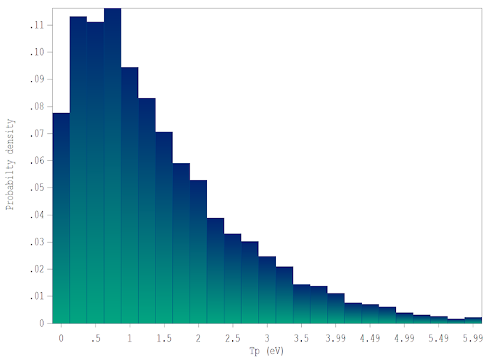
Figure 2. Initial kinetic-energy distribution of particles for kT = 1.0 eV.
LINKS
