I am consulting on a project that demands extremely accurate orbit calculations in a high magnetic field environment with saturated iron. Because the organization has another consultant with extensive experience with Maxwell 3D, the working plan is that he performs the magnetic field calculations. The resulting field values in the beam propagation region are transferred to OmniTrak in the neutral AMaze field table format. I advise on the orbit calculations, and I performed benchmark checks on the 3D field calculations with Magnum. After several rounds making sure we were representing the same system, the end result was that the Magnum results were numerically identical to the Ansoft results. There were two differences:
- * The Maxwell 3D solution took several times longer.
- * The Ansoft results had high-frequency noise.
I couldn't do much about the first problem, but I was able to alleviate the second one. OmniTrak has long included a simple command-line utility for field table preprocessing called FTabTool. I decided to expand the core of the program and to create a full-featured interactive program Mapper. Figure 1 shows a screen shot. It was frustrating to deal with field tables without being able to see them, so we included capabilities for 2D slice plots and 1D scans. Most important, we added new routines to smooth values in the field tables. The smoothing method follows the same relaxation techniques used to solve the Poisson equation. The result is that the smoothed values are actually closer to an ideal physical solution.
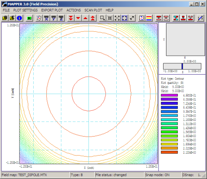
Figure 1. Mapper screen shot.
Figure 2 illustrates this effect. I prepared a field table of moderate accuracy in the space z ≥ 0.0 for a magnetic dipole and then reflected it about the midplane using the Reflection command in Mapper. The top graph shows a scan of numerical values of Bz(0.0,0.0,z). Theoretically, the variation should be parabolic. The lower graph shows the data after relaxation smoothing. The method leaves the central value almost unchanged, while a conventional smoothing algorithm would raise the central field significantly.
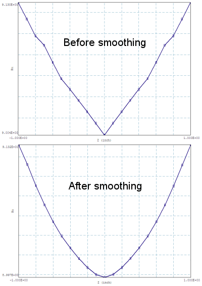
Figure 2. Mapper smooting demonstration.
LINKS
