Finite-element calculations are performed in a finite volume. Therefore, we must deal with conditions on the boundaries. Boundary conditions in Magnum program for 3D magnetic fields have some subtleties. This article is a reference on when and how to employ symmetry conditions.
For top speed and efficient use of memory, Magnum calculates a scalar quantity φ rather than the vector potential A. Section 2.1 of the Magnum manual reviews the reduced potential method. The magnetic flux density is related to the potential by
B = μ [Hs - grad(φ)],
where Hs is the applied magnetic field created by specified currents in coils. This quantity is calculated with a free-space Biot-Savart integral. To review, the quantity Hs is the contribution of coils to the magnetic flux density while the quantity grad(φ) gives the contribution of materials (e.g., iron, permanent magnets). The natural boundary condition in a finite-element calculation is that the normal gradient of the calculated quantity equals zero at the boundary:
gradn(φ) = 0.0.
The equations have two implications
- If material structures are symmetric about a plane and the currents of coils and permanent magnets are antisymmetric, then lines of B are parallel to the plane. The antisymmetric condition means that the currents created by coils and permanent magnets have opposite directions on different sides of the plane.
- Lines of B are normal to a plane where material structures, applied currents and permanent-magnet currents are symmetric. In this case, the condition φ = constant applies.
There is an important caveat with respect to the second rule. You can set φ = constant in a single plane because only the gradient is significant. The entire potential may be offset by a constant without affecting values of B. The typical choice is φ = 0.0. On the other hand, defining two planes with φ = constant changes the gradient. The rule is that only a single plane of perpendicular B may be set in a Magnum calculation.
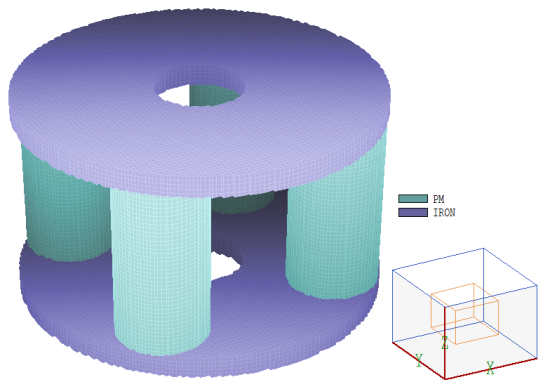
Figure 1. Test example: solenoid field with discrete permanent magnets.
A practical example will help to clarify the rules. Figure 1 shows a permanent magnet assembly to create a solenoid-type field. There are four magnets (magnetized along z) at 45°, 135°, 225° and 315° with cylindrical iron rings at the ends. The function of the system is to create an axial magnetic flux density Bz near the axis. The purpose of the calculation might be to determine the magnitude and azimuthal uniformity of the paraxial field. Here is a link to a zip file that contains the Magnum input files: example input files.
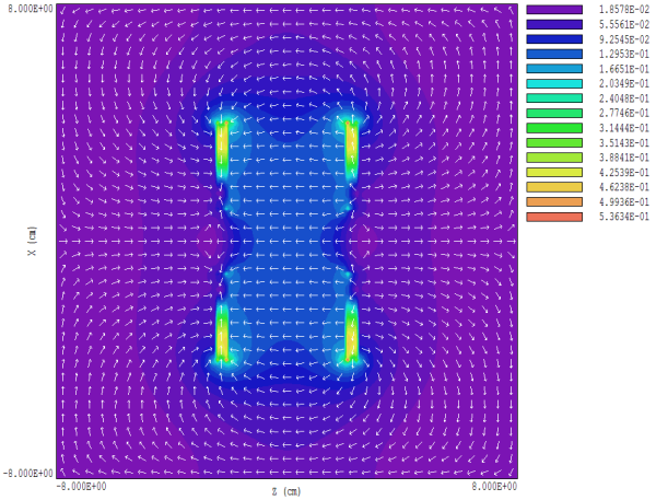
Figure 2. Lines of magnetic flux density in the plane y = 0.0.
Files with the prefix MAGNUM_SYMM111 correspond to the full solution volume. The defined objects are 1) the solution volume (air), the four magnets and the two iron rings. Figure 2 shows the direction of lines of magnetic flux density in the plane y = 0.0. Lines of B are normal to the plane z = 0.0 and are parallel to the plane x = 0.0. A plot in the plane x = 0.0 would show that B lines are also parallel to the plane y = 0.0.
The solution could be cut in half by eliminating the region z < 0.0 and using the one allowed fixed-potential boundary (φ = 0.0) at z = 0.0. The definition of the lower iron ring is removed from the mesh of MAGNUM_SYMM110 and the magnets are automatically clipped at z = 0.0. An additional region of type ZBoundDn is added and assigned the fixed-potential condition. The solution time is reduced by a factor of 2. Scans of Bz along the axis in the two solutions are numerically identical.
We could proceed another step by eliminating the region y < 0.0, setting a symmetry boundary at y = 0.0. In this case, no special provisions are needed beyond 1) eliminating negative values of y in the YMesh structure and 2) removing the two magnets at y < 0.0. Lines of B are parallel to the plane y = 0.0. This is the natural boundary condition of the finite-element condition and no special boundary condition is necessary. The files with prefix MAGNUM_SYMM100 describe this solution and give the same results. The calculation time is reduced by a factor of 4 compared to the first solution. We could go one step further, cutting the solution at x = 0.0 (one eighth of the initial solution).
How does this example relate to the symmetry rules? The physical structures (iron and permanent magnets) are symmetric about the planes x = 0.0, y = 0.0 and z = 0.0. The symbols in Fig. 3 show the directions of surface currents in the permanent magnets (out of the page and into the page). The permanent magnet current is symmetric about the plane z = 0.0, but antisymmetric about the planes x = 0.0 and y = 0.0.
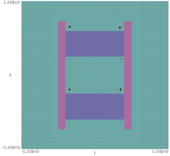
Figure 3. Cross section of the system showing the direction of surface currents in the permanent magnet.
To conclude, we could determine the symmetry type of cut planes by applying the rules. On the other hand, a physical sense of the B lines (as in Fig. 2) is usually sufficient. There are two important rules that should be emphasized:
- Even though the solution volume may cover only a portion of the space, the applied coil currents defined in Magwinder must be complete. For example, even if the solution volume covers only the quadrant x > 0.0, y > 0.0, the circular coils of a solenoid must cover 360?.
- Only one fixed-potential plane (B normal) is allowed in a solution.
LINKS
