One of the deep mysteries of the personal computer universe is how some commercial software survives when equivalent open-source packages are available absolutely free. As a long time user of OpenOffice (from the first Star Office days), I am astonished that anyone would put up with the cost and aggravation of Microsoft Office. Similarly with LibreCAD, an open-source gem. This free, actively-supported program has the power to handle the 2D design needs of probably 99% of users. We recently updated our 2D Mesh program to ensure seamless import of DXF files created by LibreCAD. This article gives a brief tutorial on interactions between two programs. In a following article, I'll discuss how to use the open-source program FreeCAD to create 3D objects as input to Geometer/MetaMesh.
The Mesh program includes a graphical shape editor with many CAD capabilities. To begin, the question is why use LibreCAD? There are two reasons:
- LibreCAD has advanced fitting features that extend beyond those of the Mesh editor.
- If you have designed a mechanical assembly in LibreCAD, it can be transferred directly to Mesh.
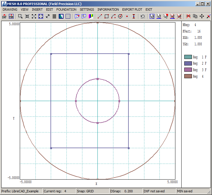
Figure 1. Mesh drawing editor, original geometry.
I'll illustrate procedures with an example of a simple electrostatic calculation, coaxial pipes with an offset dielectric. Here's a link to the Mesh input script: LibreCAD_Example.MIN. Load the file in Mesh and click on Edit mesh (graphics) to open the drawing window with the display of Figure 1. There are four regions:
- The space (FullVolume) between the pipes with a circular outer boundary of radius 5.0 cm.
- The rectangular, displaced dielectric.
- The inner circular pipe of radius 1.4 cm.
- The outer boundary of radius 5.0 cm to set a fixed-potential node condition.
The order of the regions is important. Regions over-write portions of previous regions as the Mesh script is processed. The first three regions are designated as Filled (i.e., the region number is assigned to all elements and nodes inside the bounding vectors). The fourth region is Open?? the region number is assigned only to nodes along the vectors. Clicking on Toggle fill display produces the display of Figure 2.
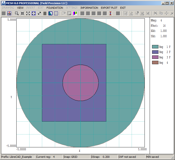
Figure 2. Mesh drawing editor, original geometry with filled display active.
To send the information to LibreCAD, use the comand Drawing/Export DXF file to produce the file LibreCAD_Example.DXF. Run LibreCAD, load the file and click on AutoZoom to create the display of Figure 3. In the list on the right, note that the vectors of Regions 1, 2, 3 and 4 have been organized into Layers 1, 2, 3 and 4.
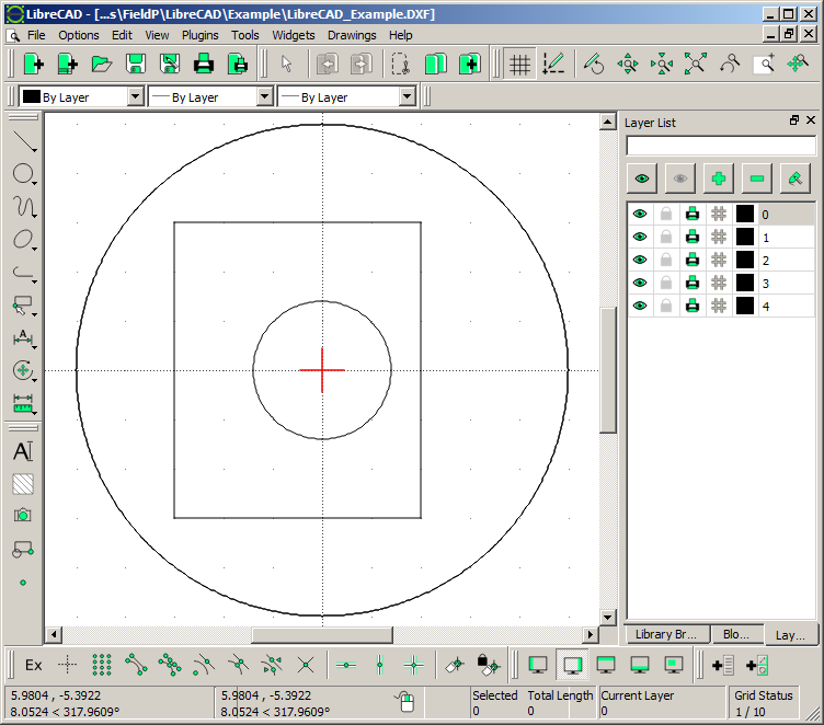
Figure 3. LibreCAD, original geometry imported.
The goal is to divide the dielectric into two sections with a complex polyline boundary and then to send the result back to Mesh. Use this procedure to ensure that the resulting layers are in the correct order to follow the over-write convention of Mesh.
- In the list on the right, highlight Layer 4. Click on Layer properties and change the name to 5.
- Similarly, rename Layer 3 to 4.
- Add a new layer and name it 3. Increase the line thickness to 0.50 mm and set the color to Blue for visibility.
To draw the boundary, click on Tools/Polyline/Polyline. Now, click on vertices to make any outline as shown in Figure 4. For the final vector, click the Close button above the drawing area. Save the DXF file LibreCAD_ExampleM.DXF.
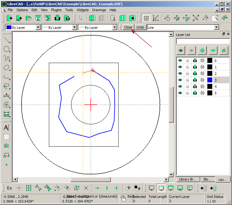
Figure 4. Drawing the polyline boundary in LibreCAD.
Back in Mesh, exit the Drawing editor. Click Create mesh/DXF file, load the file LibreCAD_ExampleM.DXF and choose Planar symmetry. The program loads the information and enters the Drawing editor with the display of Figure 5. The program detects that Region 5 contains a closed set of vectors and automatically sets it to the Filled condition. Choose Settings/Region properties and uncheck the Filled box for Region 5. Click Toggle fill display to ensure that the region order is correct. You can now click Export MIN file to create a modified mesh script with the new region:
REGION FILL Region003
 L -1.20267 2.02673 -2.27171 1.40312
 L -2.27171 1.40312 -2.11581 0.48998
 L -2.11581 0.48998 -2.31626 -0.91314
 L -2.31626 -0.91314 -1.73719 -1.93764
 L -1.73719 -1.93764 -0.11136 -2.36080
 L -0.11136 -2.36080 0.62361 -2.07127
 L 0.62361 -2.07127 1.49220 -1.84855
 L 1.49220 -1.84855 1.69265 -1.18040
 L 1.69265 -1.18040 1.73719 -0.04454
 L 1.73719 -0.04454 1.71492 1.06904
 L 1.71492 1.06904 1.33630 1.71492
 L 1.33630 1.71492 0.13363 2.47216
 L 0.13363 2.47216 -1.20267 2.02673
END
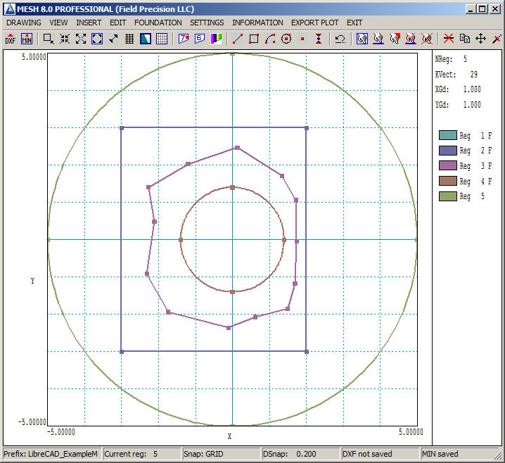
Figure 5. Revised drawing in Mesh.
The implication is that it's easy to move between Mesh and LibreCAD to make optimal use of the program functions. The example points up one useful application. If you have a complex spline curve in a drawing, you can trace it as a set of polyline vectors for input to Mesh.
LINKS
