In a another article, I discussed the basis of the H*(10) standard for radiation safety. Here, I'll continue by demonstrating techniques for shielding calculations. I'll use a published simple benchmark calculation to compare the results to several other Monte Carlo codes and to illustrate some of the advantages of GamBet. For this, I am grateful to the people at RayXpert who have made reports on a number of benchmark calculations available on the Internet. In particular, I admire their patience and fortitude in learning four other codes besides their own to make the comparisons.

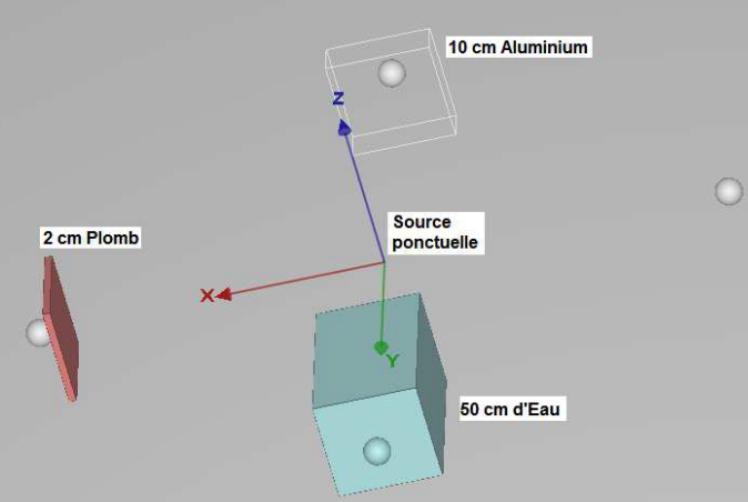
Figure 1. Geometry of the benchmark calculation taken from the RayXpert report.

Figure 1 shows the geometry taken from the report H*(10) dose rate evolution with some different shielding. Targets are located 100 cm from a Co60 point source with activity 10^9 Bq[1]. The dose at a depth of 1.0 cm was calculated for a bare target and with three shield configurations. The setup illustrates two points I made in the last article about H*(10) calculations:

1. The results are not sensitive to the detector geometry. In this case, a 4.0 cm radius sphere of tissue equivalent material is used rather than the ICRU 15.0 cm radius sphere.
2. The radiation weighting factor (Wr) is taken as unity for the photons and secondary electrons and there is no organ correction for the phantom (Wt = 1.0). In this case, the biological dose (Sv) equals the physical dose (Gy).

I limited my calculations to the bare target and to one behind a 2 cm lead shield. Here are the results reported by RayXpert. The values are given in units of µGy/hour.

             Dosimex-G  Mercurad  Microshield MCNPX RayXpert
No shielding    349        353         347      355   365
2 cm lead       143        152         141      146   149

The targets subtend only a small fraction of the solid angle surrounding the source, so it would be foolish to use an isotropic source. Instead, this is an ideal opportunity to use the GamBet Radiation Source Tool, illustrated in Fig. 2. After the user enters values in the dialog fields, the program creates a standard source file. The idea is to fill a circle of a specified radius in the direction of interest with a large, random distribution of particles. The flux assigned to each particle is calculated to represent the specified source activity. In this case, I created a distribution of 200,000 photons of energy 1.17 MeV and an equal number at 1.33 MeV. The distribution filled a circle of radius 4.0 cm at a distance of 92.0 from the source, ensuring complete irradiation of the detector. The energy deposition was symmetric about the line from the source through the detector, so I further reduced run time by using the option for cylindrical scoring in GamBet. The air region was represented by the standard Penelope dry air model and the tissue-equivalent target was represented by the custom material definition discussed in the previous article:

Material
 Name TissueEquivalent
 Component O 1.0000
 Component C 0.1940
 Component H 2.1032
 Component N 0.0390
 Density 1.00
 Insulator
End

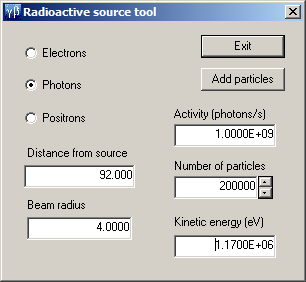
Figure 2. GamBet Radioactive Source Tool dialog.

Figure 3 shows the dose distribution calculated by GamBet for the bare detector with photons entering from the left[2]. Even for this simple case, there is quite a lot going on. The dose at the surface is lower than the peak dose in the material. This is the result of the buildup of the secondary-electron distribution. The energy loss-rate for electrons is much higher than that of photons of the same energy. The depth to reach the equilibrium dose is about 0.6 cm, hence the choice of the H*(10) measurement depth as 1.0 cm for γ rays in the MeV range. The dose rate decreases gradually through the material because of γ ray attenuation. Note the difference in the air dose rate at the entrance and exit of the target. The enhanced downstream dose rate results from electrons driven out of the material. The H*(10) dose rate determined by GamBet was 338 µGy/hour, in good absolute agreement with the values reported by RayXpert.

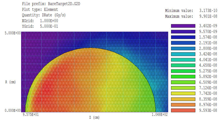
Figure 3. Dose-rate distribution for a bare target.

Figure 4 shows the dose-rate distribution with 2.0 cm lead shield placed a short distance in front of the target. The shield extends to the outer radius ? the portion irradiated by the 4.0 cm radius beam is clearly visible. The dose buildup depth in lead is shorter than the element size, so it is not visible[3]. Also, note the absence of a buildup region in the target. Most of the equilibrium secondary electron distribution from the lead crosses the small air gap and enters the target. The GamBet H*(10) prediction is 146 µGy/hour, again comparable to the values determined by the other codes. Finally, Figure 5 shows dose-rate scans along the diameter of the spherical target for the two cases. The dashed line is the H*(10) point.

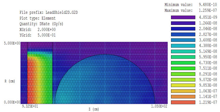
Figure 4. Dose-rate distribution for a 2.0 cm lead shield.

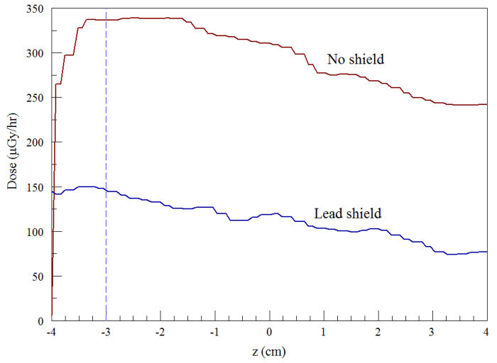
Figure 5. Dose-rate scans along a diameter of the spherical target.

One conclusion of this study is that all radiation-shielding codes give reasonable results. This is not surprising because the physics and mathematics base for Monte Carlo radiation codes is over half a century old. The question within this constraint is: why choose GamBet? Beyond its low price, GamBet has several advantages, some of which are apparent in this study:

• Zoning in GamBet is performed with conformal finite-element meshes, allowing plots such as those of Figure 3 and 4. Complex processes may enter even the simplest radiation calculations, so detailed pictures of dose distributions are essential for evaluating results.
• GamBet is fast for two reasons: 1) the code is designed to encourage division of solutions into stages and 2) the code supports efficient parallel processing. For this example, the run time with 1.6 million incident model photons (4 parallel processes with 400,000 photons each) was 7 minutes.
• The element approach in GamBet is more effective than combinatorial solid geometry to represent complex systems. The advantage is not apparent in this calculation, but is overwhelming when representing something like a human body phantom.
• Although all Monte Carlo physics engines are about equal for MeV γ rays, Penelope has far more detailed support for low-energy X-rays.
• GamBet has several advanced features, such as integration of calculated 3D electric and magnetic fields and direct coupling to electron beam and thermal transport programs.

Footnotes

[1] This article reviews the decay scheme of Co60: Modeling radioactive sources with GamBet.

[2] GamBet uses standard units of Gy/s. The conversion factor to μGy/hour is 3.6E9.

[3] The element size in GamBet determines the display resolution and the accuracy for fitting shapes, but has no effect on the physics of the radiation interactions.

[4] Contact us : techinfo@fieldp.com.

[5] Field Precision home page: www.fieldp.com.