Many processes represented by GamBet, such as the emission of bremsstrahlung photons and Compton electrons, involve interactions with atomic electrons. Particle emission may also follow from reactions within nucleii. Although GamBet does not address nuclear physics, the program can determine the histories of particles created by nuclear events. There are two types of processes: nuclear reactions and radioactivity. A nuclear reaction is a response to specific event, like fission following absorption of a neutron. On the other hand, radioactive events occur spontaneously at random times. Some nucleii are inherently unstable but in a state of local equilibrium. A transition can occur through quantum tunneling, a random process. For X-ray applications, we will limit attention to radioactivity. To begin, we'll review some nomenclature and characteristics of sources. The second part of the article deals with specific GamBet strategies.
Four types of particles may be generated in radioactive events:
- Fast electrons and positrons (beta rays)
- Photons (gamma rays)
- Heavy charged particles (protons, alpha rays,...)
- Neutrons.
This article deals with first two types. Radioactive sources of beta and gamma rays have extensive applications in areas such as medical treatments, food irradiation and detector calibration.
The activity of a radioactive source is determined by law of radioactive decay (Eq, 1). In the equation, the quantity N equals the total number of nucleii in the source. The left-hand side is the number of nucleii that decay per second. The quantity λ (with units of 1/s) is the decay constant. It depends on the energy state and quantum barrier of the nucleus. Accordingly, sources exhibit huge variations of λ. The historical units of activity for a source is the curie (Ci). One curie equals 3.7 × 10¹⁰ decays/s (approximately equal the activity of 1 gram of Ra226). The modern standard unit is the becquerel (Bq) equal to 1 decay/s (1 Bq = 2.703 × 10⁻¹¹ Ci).
We can also interpret the decay constant in terms of a single nucleus. The probability that a nucleus has not decayed after a time t is given by Eq. 2. The average lifetime (the mean of the distribution) is 1/λ. The halflife is another useful quantity. It equals the time for half of the nucleii present in a source at t = 0.0 to decay. Equation 2 leads to the expression for the halflife of Eq. 3.
In comparison to particle accelerators, the main advantage of radioactive isotopes as sources is that they do not require power input and expensive ancillary equipment (e.g., power supplies, vacuum systems,...). Many isotopes are produced by exposure in a nuclear reactor and may be relatively inexpensive when reactors are available. The disadvantages of radioactive sources are that they run continuously and produce a broad energy spectrum of electrons and positrons.
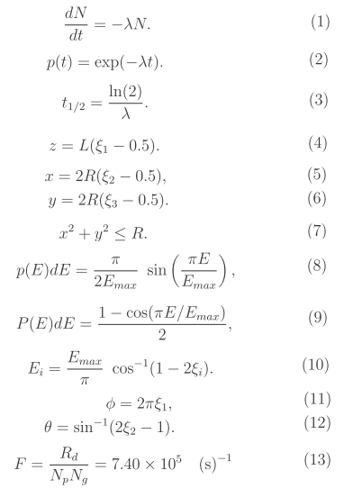
The most important nuclear processes for the production of beta and gamma rays are beta decay and electron capture. Figure 1 shows the atomic mass of the most stable isotopes as a function of atomic number Z. Isotopes above the line have an excess of neutrons their usual route toward stability is to emit a β- particle (electron), converting a neutron to a proton while preserving the number of nucleons. In other words, the nucleus changes its isotopic identity while preserving its isomer identity. Similarly, isotopes with an excess of protons emit β+ particles (positrons). Both forms of nuclear transformations are called beta decay.
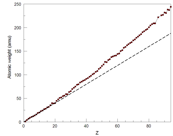
Figure 1. Atomic weight of the most stable isotopes as a function of atomic number Z. The dashed line shows the mass for equal numbers of neutrons and protons.
First, consider β- emission. There are two isotopes commonly used in research and industry: Cs137 and Co60. Nuclear processes are commonly illustrated with energy-level diagrams — Fig. 2a shows the decay scheme for Cs137. The horizontal axis represents isomer identity and the vertical axis shows energy levels. Dark lines indicate a nucleus in the ground state and light lines designate an excited state. The arrows indicate the directions of transformations. The starting point is the ground state of Cs137. The figure 30.17 years is the half-life for decay. Decay events of type β- convert the nucleus to the more stable isomer, Ba137. The arrows indicate that there are two decay paths. In 94.6% of the decays, the emission process carries off 0.512 MeV (shared between the emitted electron and an anti-neutrino) and leaves the Ba137 nucleus in an excited state. The state decays with a half-life of 2.55 minutes, resulting in emission of a 0.662 MeV gamma ray. In 5.4% of the events, the β- particle and antineutrino carry of 1.174 MeV and leaving the product nucleus in the ground state.
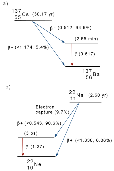
Figure 2. Energy level diagrams for the radioactive decay of Cs137 and Na22.
The emission process does not produce a single β- particle of energy 0.512 or 1.174 MeV, but rather a broad spectrum of electrons with kinetic energy spread between zero and the maximum. The reason is the condition of conservation of spin. Nucleii have spin values an integer multiple of h/2p while electrons have spin ±(1/2). For balance, an additional particle is required with half-integer spin. In his theory of beta decay, Fermi postulated the existence of neutrinos and antineutrinos, neutral particles with spin ±(1/2) and very small mass, thereby almost undetectable. In a β- decay, the available energy is partitioned between the electron, the nucleus and an antineutrino. The theory to determine the spectrum is complex — all β- decays give rise to a spectrum similar to that of Fig. 3. The spectrum is skewed toward lower energy by the effect of Coulomb attraction as the electron escapes from the nucleus. Generally, Cs137 is used as a a source of 0.662 gamma rays because the β- particles are preferentially absorbed by the source and surrounding structure and the antineutrinos pass away with no effect.
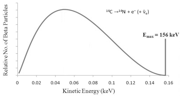
Figure 3. Distribution of electron energy for the radioactive decay of C14.
We next consider proton-rich isotopes that approach the stability line through emission of positrons. The mechanism is similar to β- emission with the exceptions that a neutrino is emitted and the positron emission spectrum shifted toward higher energies because of Coulomb force repulsion from nucleus. Figure 2b shows the energy-level diagram for Na22, a positron emitter. The halflife for all decay processes is 2.60 years. There are several decay pathways. The most likely event (90.33% probability) is that a proton changes to a neutron by emission of a positron, leaving the product isotope Ne22 in an excited state. A gamma ray of energy 1.275 MeV is released almost immediately as the nucleus relaxes to the ground state. In this case, the maximum positron energy is 0.545 MeV. In rare instances, a positron with energy 1.82 MeV is released, leaving the product nucleus in the ground state. A third process that may occur is electron capture. In 9.62% of the decays, an inner orbital electron is captured by the nucleus, again resulting in the conversion of a proton to a neutron. The Ne22 nucleus is left in the same excited state as with β+ emission, again followed by the release of a 1.27 MeV γ. The difference from β+ decay is that no positron or neutrino is emitted. Electron capture leaves a vacancy in the K or L shell of the electron cloud, so characteristic X-rays are also emitted as the atom relaxes.
This table lists useful commercial radioactive sources of electrons, photons and positrons. A common feature is a halflife of one to a few years. For isotopes with lower values, it would be necessary to produce and use them quickly. A long half life means reduced activity.
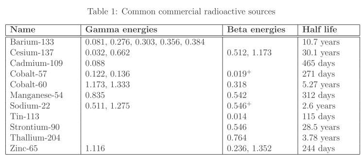
CAPTION
We'll now turn to GamBet modeling techniques, in particular how to create a particle input file to represent a radioactive source. There are some challenges:
- Particles are emitted over an extended spatial region, the volume of the source.
- Electrons and positrons have a broad energy distributions.
- Often, we want to normalize particle flux to represent a specific source activity.
Particle file creation is greatly facilitated through the use of statistical codes like R (Link to a comprehensive short course with examples on using R with GamBet).
Dealing with the finite source size is relatively easy. If the activity is uniform over the source volume, then the probability density for emission is uniform over the volume. As an example, consider a cylindrical source of length L and radius R. Given a routine that creates a random variable η in the range 0 = η = 1.0, then values of the z coordinate (along the cylinder axis) are assigned according to Eq. 4. We can use the rejection method to determine coordinates in the x-y plane. We assign coordinates by Eqs. 5 and 6 and keep only instances that satisfy Eq. 7.
With regard to energy distributions, photons from sources like Cs137 and Na22 are essentially monoenergetic. In contrast, the ß particles have an energy distribution like that of Fig. 3. In principle, thin films could be used as sources of electrons or positrons. In this case, it would be necessary to represent the spectrum and to determine the effect of energy loss in the film. The spectral shape and endpoint energy vary with the type of isotope. Chapter 10 of the reference Using R for GamBet Statistical Analysis discusses methods for creating arbitrary distributions. In practice, an exact model may not be necessary and the data may not even be available. In applications such as estimating shield effectiveness, it may be sufficient to model the β decay spectrum with a simple function like that of Eq. 8. In the equation, Emax is the maximum β energy. Taking the integral gives the cumulative probability distribution (i.e., the probability that a β has energy less than or equal to E) of Eq. 9. Values of P(E) range from 0.0 to 1.0. We can obtain the desired distribution by assigning energy from a random-uniform variable η using Eq. 10, the inverse of Eq. 9. Figure 4 shows the result with 10,000 particles having endpoint energy Emax = 0.512 MeV.
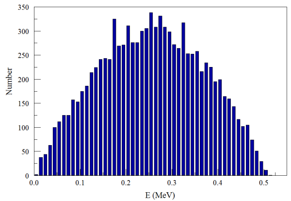
Figure 4. Generation of the spectrum of Eq. 8 with 10,000 particles using assignment from Eq. 10.
To conclude, we'll address how to create a GamBet source file to represent a given source activity. We'll follow a specific example a Co60 source with activity 10 Ci. This figure corresponds to a disintegration rate of Rd = 3.7 × 10¹¹ 1/s. Figure 5 shows an energy level diagram. The isotope decays through β- decay with a halflife of 5.27 years. Almost all events result in a excited state of the Ni60 nucleus that relaxes to the stable ground state by almost instantaneous emission of γ rays of energy 1.17 and 1.33 MeV. A source assembly typically consists of the source combined with shielding and collimators to create a directional photon flux. A goal of a calculation could be to compare radiation fluxes in the forward and reverse directions.
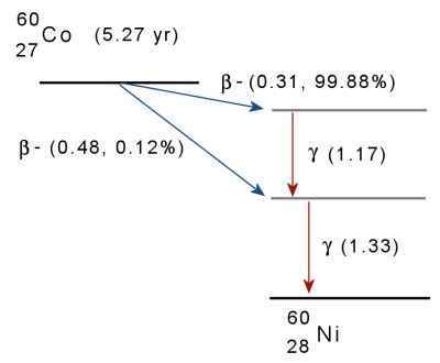
Figure 5. Energy level diagram for the radioactive decay of Co60.
We specify Np = 1000 model emission points uniformly distributed over the source volume using techniques like those discussed previously. At each emission point, we generate Ng = 500 photons of energy 1.17 MeV and Ng photons of energy 1.33 MeV. The photons are randomly distributed over 4π steradians of solid angle. Equations 11 and 12 can be used to pick the azimuthal and polar angles. In the continuous-beam mode of GamBet, each photon in the file should be assigned a flux value given by Eq. 12. In this case, GamBet gives absolute values of particle flux through and deposited dose in structure surrounding the source assembly. Note that this case is relatively simple because almost all events follow the same decay path. In the case of Cs137 (Fig. 2a), we need to multiply Rd by 0.946 to get the correct absolute flux of 0.617 MeV ? rays.
The procedure as described may be inefficient to calculate forward photon flux or shielding leakage because most of the model particles would not contribute. A simple variance reduction technique is to limit the range of solid angle dO so that photons are preferentially directed toward the measure point. The solid angle should be large enough to include the possibility of scattering from the shield or collimator. To properly normalize the calculation, the photon flux values should be adjusted by a factor dΩ/4π.
LINKS
