Our charged particle codes Trak and OmniTrak calculate electric forces on and trajectories of charged-particles that can be consider points compared to the system size (e.g., electrons, ions, ...). In this post, I'll discuss how to find electric forces on finite-size neutral dielectric or metal particles. The application that comes to mind is the forces on small dielectric objects in an electrostatic precipitator. Here, an electric field with strong gradient causes polarization of charge distribution on the object. The force is stronger on the charges on the high-field side, so there is a net force that pulls the object toward the high-field region. Because this is a second-order effect, the resulting forces may be quite small. The challenge is to construct numerical calculations with sufficient accuracy. We must find global field distributions, but maintain sufficient mesh resolution to represent small objects. In this post, I will work through an example with HiPhi. The following code features make the application feasible:
- Automatic surface integrals of the Maxwell stress tensor to find the net force on an object.
- Definition of a diagnostic surface around the object to improve the accuracy of the stress-tensor integral.
- Use of the BOUNDARY technique to employ small elements while maintaining a short run time.
If you want to follow the calculation with HiPhi, use the following links to download the the set of example files:
precipitator01.min
precipitator02.min
precipitator03.min
precipitator01.hin
precipitator02.hin
precipitator03.hin
precipitator.scr
The first figure below shows the global geometry with calculated equipotential lines. An array of rods at 50 kV (pointing out of the page) and a ground plane at the bottom are used to create an electric field with a gradient. There are symmetry boundaries at the left and right-hand sides. The object is a dielectic sphere 2.0 mm in diameter with εr = 5.6 located 1.5 cm below the center rod. The associated field perturbation is visible in the first figure.
The second figure shows a detail of the mesh near the object. The sphere has been enclosed in a cubic box with 3.0 mm sides and εr = 1.0. The function of the region is to define a second surface for evaluating the Maxwell stress tensor. In theory, integrals over the sphere and box should give the same result. In practice, the field has a smoother variation over the box so we expect a better estimate. There are two issues with the setup:
- The mesh near the object is relatively coarse in the global solution for a short run time. We would not expect good accuracy in the surface integrals.
- We must exercise judgment picking the size of the diagnostic box. The surfaces should be relatively close, within the region of field perturbations generated by the sphere. If the surfaces are too far away, the tiny effect of the sphere would be lost in numerical noise.
Here are the contents of an analysis script to find forces on the sphere along (Region 4) and the assembly of the sphere and diagnostic box (Regions 4 and 5):
OUTPUT Precipitator01
INPUT Precipitator01.HOU
FORCE 5
FORCE 4 5
ENDFILE
The Maxwell routine returns a surface area of 1.2382E-05 m2 compared to the theoretical value of 1.2566E-5 m2. The difference reflects the faceted approximation to the spherical shape. The calculated force is Fy = 2.9902E-06 N on the spherical surface and Fy = 5.1111E-06 N on the diagnostic surface. The large difference results from inaccurate field interpolations on the coarse mesh. We can gauge the accuracy by repeating the calculation with εr = 1.0 for the sphere. In principle, the force should be zero. In this case, the integral on the diagnostic gives Fy = -7.0565E-07. Therefore, we expect the surface integral on the box is in error by ~10-20%.
A useful feature in HiPhi is the ability to construct microscopic solutions using the global solution to set Dirichlet boundary conditions. For this case, I made a microscopic solution in a cubic box 2.0 cm on a side centered on the dielectric object. The third figure below shows calculated equipotential lines in the plane z = 0.0 cm for an element size of 0.2 mm. In this case, the calculated surface area of the sphere is 1.2637E-05 m2, close to the theoretical value. The calculated forces are Fy = 5.7093E-06 N (sphere) and Fy = 6.9591E-06 N (diagnostic box). With εr = 1.0 in the sphere, the residual force on the box is Fy = -8.5519E-08 N, only about 1.2% of the calculated force. I expect that the value 6.96E-6 N is close to the correct answer. If your life depended on the number, you could repeat the calculation with reduced elements near the box.
In any calculation, we always must consider the possibility that we have made an error in the setup. It is a good practice to check that the numerical result is reasonable. As an alternate approach, we can use the method of virtual work. In an electrostatic system with specified voltages, if we displace an object a distance Δd and observe a change in total field energy ΔW, then the force component along the direction of displacement is F = ΔW/Δd. To apply the method, I constructed a second microscopic solution where the sphere and diagnostic box were displaced +1.0 mm in y. I used the Full analysis function in PhiView to find the total system field energy 5.86829E-05 J. The field energy for the original solution was 5.86829E-05. Dividing the difference of 8.1E-9 J by 0.001 gives the vertical force estimate Fy = +8.1E-6. This value is within the ballpark. We would not expect high accuracy because the energy method depends on extremely small differences between numbers. Another disadvantage of the virtual work method is that it requires two calculations.
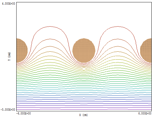
Electrostatic force, macroscopic solution.
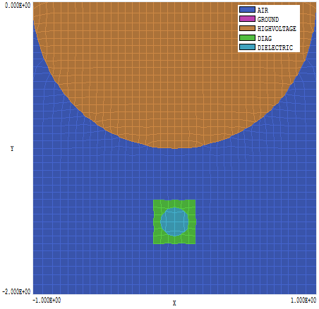
Electrostatic force, macroscopic mesh detail.
LINKS
