In the Track mode (single-particle orbits), OmniTrak has long had the capability of including temporal modulations of electric and magnetic fields to approximate RF fields in the long-wavelength limit. For electric fields, the procedure has been to multiply potential values by a modulation function M(t). Recently, I have worked on an application to design an RF ion extractor with a biased control electrode. This situation is fundamentally different. When applying a simple modulation, the assumption is that the spatial field distribution is self-similar. The only change with time is the normalization of the field solution. This type of field solution involves a reference potential (ground) and one independent value of the time-varying voltage.
With two independent time-varying electrode voltages, the spatial distribution of the field changes at each instant. Clearly, it would be impractical to solve for the three-dimensional electric field at each integration step of a particle orbit. Fortunately, there is a simple way to find the time-varying field when there are two independent voltages. We can understand the method with reference to the field solution illustrated in Figure 1. The simple three-electrode system has a ground plane at the bottom. Independent voltages may be applied to the electrode at the top left (V1) and right (V2). We can construct two normalized base solutions: solution S10 has V1 = 1.0 V and V2 = 0.0 V while solution S01 has V1 = 0.0 V and V2 = 1.0 V. In the absence of nonlinear materials, the set of all possible electrostatic solutions with arbitrary voltages V1 and V2 may be generated by a linear combination of the base functions:
S = V1*S10 + V2*S01.
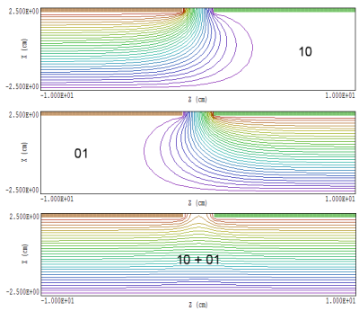
Figure 1. Base solutions, three-electrode system.
To illustrate, the bottom solution in Figure 1 is the sum of the base functions. The same solution would follow from a direct HiPhi solution with V1 = V2 = 1.0 V.
The following procedure is used for modulated dual-voltage solutions in OmniTrak:
- Prepare two base electrostatic solutions with HiPhi using the same mesh. One or more reference electrodes in both solutions are grounded (φ = 0.0 V). In the first solution, one electrode (or set of electrodes) has V1 = 1.0 V and the other has V2 = 0.0 V. The voltages levels are reversed in the second solution.
- Load the first solution with the EFIELD3D command. The program reads the mesh characteristics as well as the potential values at all nodes, φ1(i,j,k). A normalization factor may be included in the command to set the amplitude V1 in solution S10.
- Load the second solution with the new EFIELD3D2 command. In this case, OmniTrak checks that the mesh is identical to the previous one and stores the potential values φ2(i,j,k). Again, a normalization factor may be used to set the amplitude V2 for S01.
- The command MODFUNC E is used to define a modulation function M1(t) for S10, while the command MODFUNC E2 sets the modulation function M2(t) for S01.
During orbit tracking, the program uses electrostatic potential values of the form
φ = M1(t)*S10 + M2(t)*S01,
as input to the electric field interpolation routine. Because much of the computational work involves identification of the element occupied by the particle, there is little change in the orbit tracking time penalty for a dual-voltage solution.
We can track a proton through the solution shown in the first figure to demonstrate the procedure. The Field section of the OmniTrak script includes the following commands:
EFIELD3D: ThreeElect01.HOU 100.0
MODFUNC(E) > sin(1.2566E7*$t)
EFIELD3D2: ThreeElect02.HOU 200.0
MODFUNC(E2) > sin(3.1416E7*$t)
The left-hand electrode has a sinusoidal variation at 2.0 MHz with amplitude 100 V. The peak electric field far from the gap is Ex = -2000 V/m. The voltage on the right-hand side varies at 5.0 MHz with amplitude 200 V (Ex = -4000.0 V/m). A 250 eV proton moving in z is injected near the left-hand boundary. The transit time over the 20.0 cm distance is about 1.0 μs. The commands
LISTON 1
LISTTYPE EField
specify an electric-field listing along the particle trajectory. Figue 2 shows the resulting electric field experienced by particle as a function of axial position.
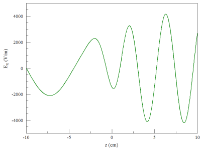
Figure 2. Voltage level along a protion trajectory.
LINKS
