I recently completed a consulting project to design an electron-beam scanning system with difficult requirements: 1) dual axis scanning, 2) large beam diameter, 3) large deflection angle and 4) short magnet length. The conditions demanded a large magnet aperture, precluding a conventional dipole with a narrow gap. Ultimately, I used two cosine coils with 90° angular separation.
The ideal cosine coil is a free-space winding on a cylinder of radius R with infinite length in z (the initial direction of beam propagation). The winding produces a uniform dipole field in the region r < R if the current density density varies as jz ~ cos(θ). The actual system differs from the ideal in two respects:
- The current is produced by discrete windings with spacings chosen to approximate the current-density variation.
- The coil has finite axial length
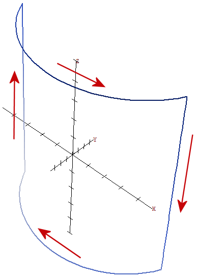
Figure 1. Single winding of a finite cosine coil.
Figure 1 shows one turn of a coil assembly along with a reference coordinate system. There are two axial line segments that carry oppositely-directed currents. The current must follow arcs on the end to keep the beam aperture free. There are two tasks to create a Magnum model:
- Determine the best positions for the discrete windings.
- Build a coil definition file for MagWinder to generate the applied-field current elements.
Regarding the first task, we need a set of angular positions θ(n) in the x-y plane such that the angular spacing between points is proportional to 1/cos[θ(n)]. An exact solution involves a transcendental equation, so I used an iterative method. It may not be the best method, but it works. I constructed a spreadsheet that had two control parameters: NStep is a large integer and Ncoil equals half of the desired number of windings. The sheet had the following columns:
- Column 1: θ(n) is the angle in radians, where θ(1) = 0 and θ(n+1) = θ(n) + Δθ(n).
- Column 2: Δθ(n) is an angular interval (in radians) weighted by 1/cos[θ(n)], where Δθ(n) = (π/2)/[NStep*cos(θn)].
- Column 3: the angle Δθ in degrees.
- Column 4: NEntry, the accumulated number of angular intervals.
- Column 5: NEntry/NCoil.
The procedure is to adjust NStep until NEntry/NCoil has an integer value at θ = 90°. For example, if the value is 100 and NCoil = 12, then choose angular values Δθ(n) at NEntry = 50,150,...,1150.
The MagWinder utility produces a large set of differential current elements from coil specifications to define the applied field in Magnum. In this case, each winding includes two LINE and two ARC models. Initially, I attempted to calculate coordinates and build the Magwinder script with a text editor. Finding that a 24-turn coil occupied almost two hours of work, I decided to automate the process. I wrote a Perl script (cosine_coil.pl) to generate a complete coil assembly in MagWinder text format automatically. The input parameters are the set of angles in the x-y plane, the coil radius R and the axial half-length, L/2. The 24-turn coil shown in the second figure occupied 460 lines in the CDF file and resolved into 2512 current elements. In the final assembly, I included a ferrite shield to limit the extent of the field and to reduce the required A-turns. The final assembly shown is quite different from both an ideal cosine coil and a sharp-edged bending magnet. In particular, field lines bulge out the axial ends. Nonetheless, OmniTrak calculations showed that the device could provide large deflections (> 35°) with 1) seperable focusing in the deflection and non-deflection planes and 2) a smooth transformation of the beam profile.
The following resources are available for download if you want to model cosine coils:
- The sample spreadsheet cosine_coil.xls to determine winding positions.
- The Perl script cosine_coil.pl to generate Magwinder input. (Note that the script file is named cosine_coil.txt to prevent conflicts with browsers.)
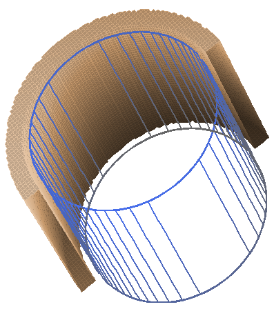
Figure 2. Cosine coil assembly with ferrite shield (cutaway view).
LINKS
