EStat and HiPhi can determine dielectric-type and conductive-type electrostatic solutions. As discussed in the program manuals, both types involve a solution to the Poisson equation. There are two differences in conductive solutions:
- The relative dielectric constant εr is replaced with the conductivity σ.
- There is no accumulation of space-charge, ρ = 0.0.
A customer recently suggested a good EStat accuracy test involving a conductive solution, so I prepared a demonstration calculation. I will describe it this article because it gives a good opportunity to review features of conductive solutions.
Figure 1 shows the geometry of a planar (infinite extent out of the page) EStat calculation. Most of the volume is filled with a medium (CONDUCTOR) with electrical conductivity σ = 1.0 S/m. A large insulator (INSULATOR01) separates two electrodes (ELECTRODELEFT at +1.0 V and ELECTRODERIGHT at -1.0 V). I added a second insulator (INSULATOR02) to introduce a significant asymmetry between the electrodes. The accuracy test is the following: no matter what geometry is chosen, the current out of one electrode should exactly equal the current into the other electrode. This condition follows because no current enters or leaves the solution volume.
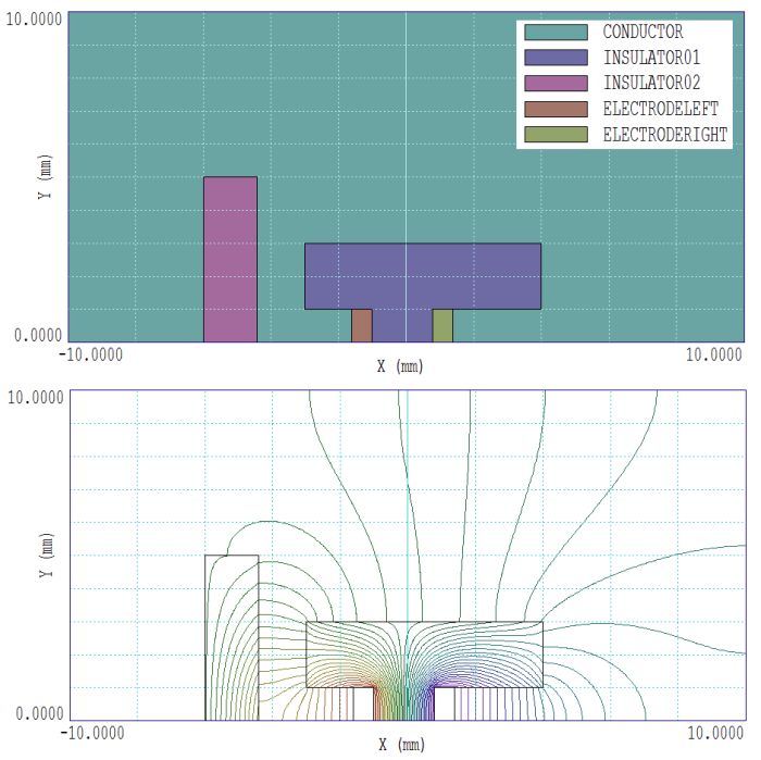
Figure 1. Calculation with internal insulators approximated with regions of low conductivity.
The solution (CONDTEST01) has two features of interest:
- In dielectric-type solutions, application of the Neumann boundary condition (the natural boundary of finite-element solution) around the entire solution volume is usually non-physical. Such a condition would apply to a periodic set of solution volumes, infinite in both directions. On the other hand, an extended Neumann boundary is appropriate in most conductive solutions. The condition that the component of electric field normal to the boundary is zero. implies that the current must flow parallel to the boundary. In other words, the Neumann condition implies that the conductive medium is enclosed in an ideal insulating container. Note that the equipotential lines in Fig. 1 intersect the boundaries at right angles so that the normal component of electric field is zero.
- The computational method to solve the Poisson equation is invalid if σ = 0.0, so we must choose a relatively low value of conductivity to represent the internal insulators. I picked σ = 10-6. Note that extremely low values impede the numerical convergence and can lead to inaccurate solutions.
The bottom part of Fig. 1 shows calculated equipotential lines. Note that, despite the system asymmetry, the electric field values on the surfaces of the two electrodes are equal. With regard to calculating total current, its always best to avoid integrals over the surfaces of electrodes with sharp edges. I elected to use the line integral function in the EStat analysis menu to find the integral of total normal linear current a short distance from each electrode surface. Here is an analysis script that I prepared to perform the calculation automatically:
Output CondTest.DAT
Configuration c:\fieldp\tricomp\estat_conductive.cfg
Input CondTest01.EOU
LineInt -1.65 0.00 -1.65 1.00
LineInt -0.00 0.00 0.00 1.00
LineInt? 1.45 0.00 1.45 1.00
Input CondTest02.EOU
LineInt -1.65 0.00 -1.65 1.00
LineInt? 1.45 0.00 1.45 1.00
ENDFILE
The calculation showed a total line current of -0.2052514 A/m on the left side and -0.2052518 on the right, equal to within 2.0 × 10⁻⁶. The current through the central (approximated) insulator was only 1.0 × 10⁻⁶ A/m.
The solution geometry has the feature that all internal insulators contact the solution-volume boundary. In this case, we can an take alternate approach — defining a complex boundary for the conducting medium that excludes the insulators (COND_TEST02). In this case, the Neumann condition applies around the entire boundary except the portion occupied by the electrodes (Dirichlet boundary). Figure 2 shows the geometry and calculated field lines. In principle, no approximation is required for the internal insulators so that solution is ideal. The disadvantage is that it gives no information about the field distribution inside the insulators. For comparison, a line integral gives -0.2052507 A/m on the left-hand side and -0.2052511 A/m on the right (again a difference of about 2.0 × 10⁻⁶). The solution confirms that the choice σ = 1.0 × 10⁻⁶ was sufficiently small to give accurate results. For extra credit, try this solution with a spatial variation of conductivity. The electrode currents will still be equal.
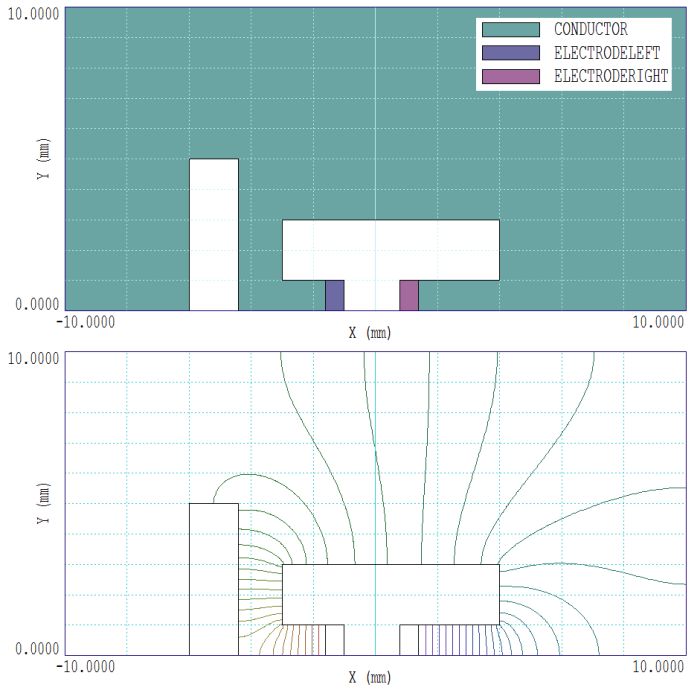
Figure 2. Calculation with a shaped Neumann solution-volume boundary to define the internal insulators.
LINKS
