EStat and HiPhi can find electrostatic solutions for collections of ideal dielectrics or ideal conductors. I often get questions about how to deal with calculations where some of the materials act like dielectrics and some like conductors. The EStat and HiPhi manuals give some brief guidelines. In this post, I wanted to give a more complete description of the underlying theory and solution strategies.
Let's begin with definitions. An ideal dielectric is a material like lucite, teflon or alumina which has an effectively infinite resistivity. We can ignore the conduction of real current, even for long voltage pulses. At the other extreme is the ideal conductor. Here, the flow of real current is much larger than the flow of displacement current. If Δt is the voltage pulse length, then we can write the condition for the dominance of real current as:
Δt ≫ εr ε0/σ,
where εr is the relative dielectric constant and σ is the conductivity. (As in all posts, I am using SI units.) For a static solution, the voltage distribution in all materials with non-zero σis determined by the flow of real current.
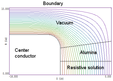
I can best illustrate the solution strategy with an example. The illustration below shows a dummy resistive load to test a pulsed-power generator. The system has cylindrical symmetry — it is a figure of resolution about the z-axis along the bottom. The outer boundary is at ground potential. The high-voltage electrode is connected to a resistor consisting of an alumina envelope filled with a water solution of copper-sulphate. We assume that the conductivity of the solution is high-enough to satisfy the above equation for the voltage pulselength. In this situation, the water-solution acts like an ideal conductor and the other materials (alumina and vacuum) are ideal dielectrics.
The calculation strategy follows from two observations:
- The voltage distribution in the water is determined by the flow of real current and is independent of the voltage distribution in the surrounding structures.
- At the boundary between the water and insulator, there is only a parallel component of real current. Because j = σE, the normal component of electric field at the boundary is zero.
We can satisfy the two conditions if carry out a dielectric-type solution and assign a value of relative dielectric constant to the water region that is much larger than the dielectric constants of the surrounding insulators.
The following values were used for the calculation shown in the figure:
Vacuum: εr = 1.0
Alumina: εr = 7.8
Water solution: εr = 1000.0
The equipotential lines show that the electric field is uniform in the water-solution. This field distribution provides a boundary condition for the electric field in the surrounding dielectrics.
Please contact us for the EStat input files for the example. As an exercise, check the field distribution when the radius of the water solution varies with z.
In summary, to represent an ideal conductor in a dielectric solution, use a relatively high value of εr. If the solution involves two connected conductive regions with, for example, σ1 = 1.0 S/m and σ2 = 2.0 S/m, then use σ1 = 1000.0 and σ2 = 2000.0.
Please use these links if you want more information about EStat or HiPhi:
http://www.fieldp.com/estat.html
http://www.fieldp.com/hiphi.html
LINKS
