When we have inquiries about automatic control of calculations, my stock reply has been that it's easy, just write a Perl script. After many years of such replies, I thought the time might be ripe to show that this is actually possible. In this note, I'll work through an example that illustrates the main operations in controlling our software from a script:
- Creating input scripts with variable information.
- Running programs and waiting for them to finish.
- Performing analysis operations.
- Abstracting data and recording it in a readable format.
I will work with the Perl scripting language. Although it is somewhat challenging to learn, Perl has several advantages:
- A full distribution for Windows is available at no charge from ActiveState.
- There is extensive documentation on the Internet and several useful references, such as T. Christiansen and N. Torkington, Perl Cookbook (O'Reilly and Associates, Sebastopol, 1998).
- It enables control of every aspect of your PC.
- It is very powerful. You can advance beyond the level of this demonstration to build full optimization controllers.
The example Perl program controls the calculation discussed in the note Floating potential of an open region. The script performs the following sequence of operations:
- Calculate the mesh.
- Generate 20 EStat solutions with different values of the grid potential.
- Find the field energy for each solution.
- Collect the results in a formatted list.
- Clean up the directory.
Here are links to the example input files
Mesh input file: perl_demo.min
Template EStat input file: perl_demo.ein
EStat anlysis script: perl_demo.scr
Controlling Perl script: run_control.pl
I'll discuss some of the entries in the Perl file:
1) This command in Section B runs Mesh to create the mesh file.
$status = system("c:/fieldp/tricomp/mesh",$FilePrefix);
The Perl script waits for the completion of the task before proceeding, so the MOU file will be available for the electrostatic calculations. The section also illustrates how to issue an error message and to stop the run if the task was not successful.
2) Section C is a loop through potential values. I prepared a template script perl_demo.ein where the @ symbol was used in place of a numerical value for the potential of Region 4 (the grid). The following code extract opens the template file and writes a temporary script with the current value of potential $V substituted for @:
open (InFile,"<",$FileNameIn);
open (OutFile,">",$FileNameOut);
while (<InFile>)
  {
  $Line = $_;
  $Line =~ s/@/$V/;
  print OutFile $Line;
}
The script then runs EStat with the input script. The result is a series of output solution files with names of the form perl_demo01.eou, ..., perl_demo20.eou.
3) In Section D, this statement runs an EStat script that writes volume integrals for the 20 solutions to the file perl_demo.dat.
$status = system("c:/fieldp/tricomp/estat","perl_demo.scr");
4) Finally, Section E of the script reads through all lines of perl_demo.dat, picks lines that contain the string "Energy:", and writes then to the file summary.dat:
open (InFile,"<","perl_demo.dat");
open (OutFile,">","summary.dat");
$V = $VMin;
while (<InFile>)
  {
  $Line = $_;
  if (m/Energy:/s)
    {
    print OutFile "Voltage:  $V    $Line";
    $V = $V + $dV;
    }
  }
close InFile;
close OutFile;
Here are the contents of the final output file:
Voltage:  2000     Energy:   4.0191E-04 J
Voltage:  2400     Energy:   3.8856E-04 J
Voltage:  2800     Energy:   3.7807E-04 J
Voltage:  3200     Energy:   3.7046E-04 J
Voltage:  3600     Energy:   3.6572E-04 J
Voltage:  4000     Energy:   3.6384E-04 J
Voltage:  4400     Energy:   3.6484E-04 J
Voltage:  4800     Energy:   3.6871E-04 J
Voltage:  5200     Energy:   3.7545E-04 J
Voltage:  5600     Energy:   3.8507E-04 J
Voltage:  6000     Energy:   3.9755E-04 J
Voltage:  6400     Energy:   4.1290E-04 J
Voltage:  6800     Energy:   4.3113E-04 J
Voltage:  7200     Energy:   4.5223E-04 J
Voltage:  7600     Energy:   4.7619E-04 J
Voltage:  8000     Energy:   5.0303E-04 J
Voltage:  8400     Energy:   5.3274E-04 J
Voltage:  8800     Energy:   5.6532E-04 J
Voltage:  9200     Energy:   6.0078E-04 J
Voltage:  9600     Energy:   6.3910E-04 J
Voltage:  10000    Energy:   6.8029E-04 J
I used the values to create the plot of Fig. 1. In conclusion, this example gives just a few suggestions and templates for automatic control of Field Precision software. With the power of Perl, the possibilities are endless.
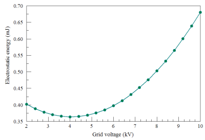
Figure 2. Electrostatic field energy versus grid voltage
LINKS
