One of the outstanding features of our software is the use of input scripts, a classic feature of early programs that we have updated. The term script refers to a text file of input data for a program run. Figure 1 shows the role of input scripts in Field Precision software. Years ago, the primary input method for technical programs followed the sequence in the middle of the illustration. A user would employ a text editor (or a punch card machine, if we go far enough back) to create the set of instructions passed to the program. Early scripts were rigid in the order and syntax of instructions and documentation was often sparse. As a result, the script method acquired a bad reputation.
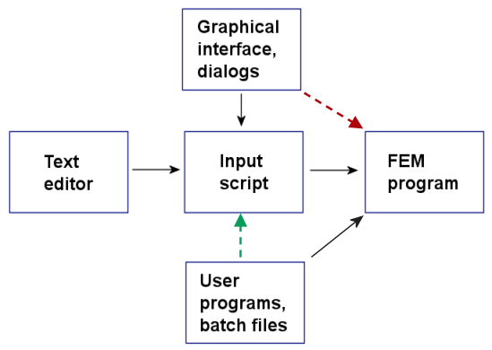
Figure 1. Input options for Field Precision technical programs.
Users welcomed the appearance of graphical-user interfaces. Here, the programs remembered the instruction syntax and provided setup guidance. Most modern technical programs follow the sequence show by the red arrow in Fig. 1. The user sets controls or fills in fields, and the data is passed directly to the program. In contrast, Field Precision programs follow a two-step process where the interactive routines produce a text script which is then read by the program[1]. There are several reasons why we have chosen this route:
- Compact scripts are an effective method for archiving run setups and exchanging them with colleagues.
- Input information is transparent to the user.
- Scripts provide expanded input options.
We will concentrate on the third advantage in this article.
Field Precision programs offer two alternatives to the graphical-user-interface. Direct editing of the script is useful for checking values and making small changes (e.g., moving objects, modifying material properties,...) without the need to negotiate the GUI. In the past, our programs have had a limited capability for control through Windows batch files and external programs (e.g., Python scripts,...), indicated by the black arrow in Fig. 1. All of our programs had the capability to run from the command line or to be called by an external program. The single pass parameter was the name of the input script.
The change described in this article, represented by the green arrow in Fig. 1, applies to the all 2D and 3D Field Precision programs. Batch files and external programs can now control how the technical program interprets variable quantities in the input script. The easiest way to describe the feature is to follow an application example. Figure 2-top shows the geometry of a test calculation, the magnetic field of a cylindrical coil in an air volume. Finite-element solutions are performed in a finite-volume and require a specified condition on the boundary. The most boundary for magnetic-field calculations is a Dirichlet condition (constant vector potential). In the case, the boundary acts like a perfectly-conducting wall (Fig. 2-bottom). The purpose of the study is to determine how large the boundaries must be to approach the infinite-space result.
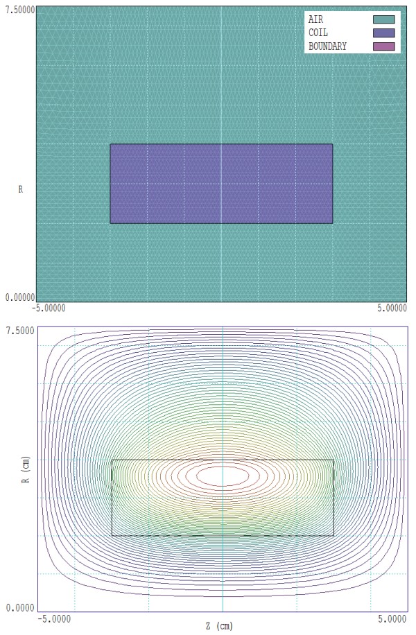
Figure 2. Test calculation, magnetic field of a cylndrical coil in space. Top: Mesh. Bottom: Calculated field lines.
The procedure is to compute several solutions with different boundaries, comparing the values of the field at the center of the coil, Bz(0,0). The mesh input script BATCHCONTROL.MIN looks? like this:
* -------------------------------------------------------
GLOBAL
 ZMESH
  %1 -3.5 0.2
  -3.5 3.5 0.1
  3.5 %2 0.2
 END
 RMESH
  0.0 4.5 0.1
  4.5 %3 0.2
 END
END
* -------------------------------------------------------
REGION FILL AIR
 L %1 0.00000 %2 0.00000
 L %2 0.00000 %2 %3
 L %2 %3 %1 %3
 L %1 %3 %1 0.00000
END
* -------------------------------------------------------
REGION FILL COIL
 L -3.00000 2.00000 3.00000 2.00000
 L 3.00000 2.00000 3.00000 4.00000
 L 3.00000 4.00000 -3.00000 4.00000
 L -3.00000 4.00000 -3.00000 2.00000
END
* -------------------------------------------------------
REGION BOUNDARY
 L %1 0.00000 %2 0.00000
 L %2 0.00000 %2 %3
 L %2 %3 %1 %3
 L %1 %3 %1 0.00000
END
* -------------------------------------------------------
ENDFILE
In the GLOBAL section, notice that there is region of small elements around the coil and then larger elements to the outer boundaries. Further, note the symbolic representation of the boundary limits, a convention familiar to users of Windows batch files. The symbol %1 represents ZMin, %2 represents ZMax and %3 represents RMax.
The calling batch file has the following content:
START /B /WAIT C:\fieldp_pro\tricomp\mesh.exe C:\Simulations\BatchControl -5.00 5.00 7.50
START /B /WAIT C:\fieldp_pro\tricomp\permag.exe C:\Simulations\BatchControl.PIN
START /B /WAIT C:\fieldp_pro\tricomp\permag.exe C:\Simulations\BatchControl.SCR
START /B /WAIT C:\fieldp_pro\tricomp\mesh.exe C:\Simulations\BatchControl -6.00 6.00 9.00
START /B /WAIT C:\fieldp_pro\tricomp\permag.exe C:\Simulations\BatchControl.PIN
START /B /WAIT C:\fieldp_pro\tricomp\permag.exe C:\Simulations\BatchControl.SCR
START /B /WAIT C:\fieldp_pro\tricomp\mesh.exe C:\Simulations\BatchControl -7.00 7.00 10.50
START /B /WAIT C:\fieldp_pro\tricomp\permag.exe C:\Simulations\BatchControl.PIN
START /B /WAIT C:\fieldp_pro\tricomp\permag.exe C:\Simulations\BatchControl.SCR
START /B /WAIT C:\fieldp_pro\tricomp\mesh.exe C:\Simulations\BatchControl -8.00 8.00 12.00
START /B /WAIT C:\fieldp_pro\tricomp\permag.exe C:\Simulations\BatchControl.PIN
START /B /WAIT C:\fieldp_pro\tricomp\permag.exe C:\Simulations\BatchControl.SCR
...
The file seems verbose, but it is mainly copy-and-paste from a template prepared with the Create task button of the TriComp program launcher. The interesting lines are those that call Mesh. The first pass parameter is the input script listed above. The three additional string parameters give numerical values for the variables %1, %2 and &3. There are multiple solutions with expanding boundaries with the constraint RMax = 1.5 ZMax. The two commands that follow run PerMag with the modified mesh and then execute the analysis script BATCHCONTROL.SCR. This file has the following content:
INPUT BatchControl.POU
OUTPUT BatchControl.DAT Append
POINT 0.0 0.0
ENDFILE
The Append specification in the second command ensures that all the data will be added in sequence to a single output file.
The full set of runs is generated in about two seconds by executing the batch file. The data are available as text entries in BATCHCONTROL.DAT. Figure 3 shows a plot of the results. The dashed line is the theoretical result for an infinite space.
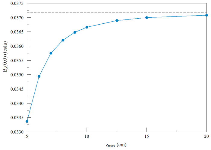
Figure 3. Central field of a cylindrical coil as a function of the boundary dimension. The dashed line is the theoretical result for infinite space.
You can imagine the infinite possibilities for automation. For example, suppose we wanted to do a more intensive analysis of each solution and record the results in a separate file. In this case, the calling batch might look like this:
...
START /B /WAIT C:\fieldp_pro\tricomp\mesh.exe C:\Simulations\BatchControl -6.00 6.00 9.00
START /B /WAIT C:\fieldp_pro\tricomp\permag.exe C:\Simulations\BatchControl.PIN
START /B /WAIT C:\fieldp_pro\tricomp\permag.exe C:\Simulations\BatchControl.SCR BatchControl02.DAT
...
and the OUTPUT command in the analysis script would become
OUTPUT %1
LINKS
