I had an inquiry from a user interested in microwave heating of dielectric samples in a air-filled waveguide. The application presented a good use of the capability to couple Aether solutions to HeatWave, so I wrote and tested a set of template input files.
In the solution, the sample was suspended at the center of a rectangular waveguide that carried a traveling wave in the TE10 mode. The wave was polarized with Ey and the guide had dimensions a = 10.0 cm along x and b = 8.0 cm along y. The sample was a cylinder of radius 2.0 cm and height 3.0 oriented as shown in Fig. 1. Heating occurred via capacitive currents driven in the resistive object. The mesh had cubic elements with sides 0.1 cm for good resolution of the sample volume.
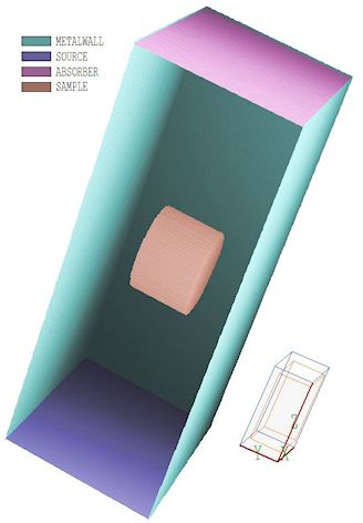
Figure 1. Mesh for the calculation showing the waveguide walls, the source and absorbing layers and the heated sample.
The first task was to generate a good approximation to a TE10 mode solution. For guidance, I followed Chap. 9 of the Aether Tutorial Manual, TE10 mode in a rectangular waveguide. The cutoff frequency was
f0 = c/2a = 1.5 GHz.
At a working frequency of f = 2.0 GHz, the vacuum wavelength was λ0 = 15.0 cm and the ratio of the group velocity to the speed of light was:
vg/c = v[1 - (λ0/2a)2]1/2 = 0.6614.
I modeled a waveguide section of length 20.2 cm. The mesh was built by defining a metal box with dimensions Wx = 10.2 cm, Wy = 8.2 cm and Wz = 20.2 cm. The interior was created by over-writing with an air box of dimensions Wx = 10.0 cm, Wy = 8.0 cm and Wz = 20.2 cm. Ideal absorbing layers of thickness Wz = 0.1 cm filled the entrance and exit. The entrance layer carried a current density
Jy = (1.0 × 10⁴) cos (0.3142 x).
When waves are normally incident, the conductivity for a matched absorbing layer is given by reference[1] as:
σ = 1/η Wz(S/m),
where η is the characteristic impedance of the adjacent medium (377.3Ω for air). As discussed in the Aether tutorial, the value must be adjusted by vg/c for modes in a waveguide. The calculated value is σ = (0.6614)(2.654) = 1.756 S/m. Figure 2 shows a plot of |E| in the plane y = 0.0 cm with the properties of the sample set to those of air. For an ideal traveling wave, the magnitude of the electric field should be constant in z.
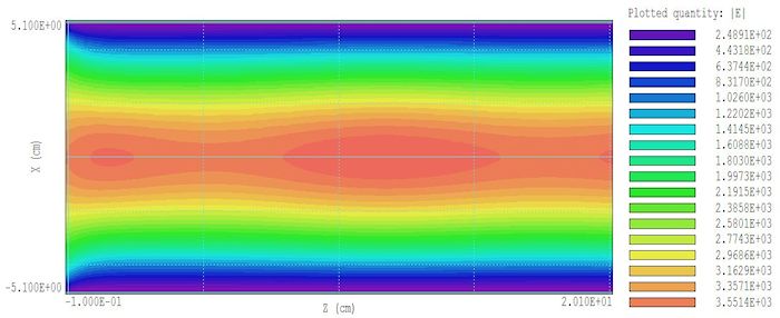
Figure 2. Plot of |E| for the TE10 mode with no sample.
If the heating is to be effective and the finite-element calculation accurate, the electric field should penetrate the object rather than concentrate in a thin surface layer (i.e., field exclusion). I picked the following material properties: εr = 1.8, μr = 1.0 and σ = 0.5 S/m. Figure 3 shows the altered electric field when the sample is present. A substantial fraction of the electromagnetic power is reflected, resulting in an upstream standing-wave component. About half the power is transmitted as a downstream traveling wave and half is absorbed by the sample (19.2 W). Figure 4 shows the spatial variation of time-averaged power density in the sample in the plane x = 0.0 cm. The peak value is p = 1.644 × 10⁶ W/m3.
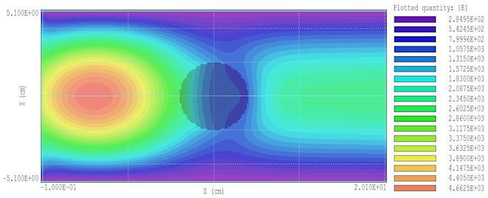
Figure 3. Plot of |E| for the TE10 mode with the sample present.
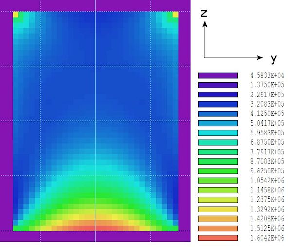
Figure 4. Power-density in the sample, plot in the plane x = 0.0 cm.
The next step was to set up a HeatWave solution using the output from Aether as a thermal source. The goal of the calculation was to investigate heating of the sample and the surrounding air. Thermal effects in the virtual source and absorber layers are not of interest. Therefore, these regions along with the metal wall were set to the fixed-temperature condition T = 0.0 oC. The sample had thermal properties k = 0.02 W/m2-oC, Cp = 2000.0 J/kg-oC and ρ = 1000.0 kg/m3. The air region has properties k = 0.024 W/m2-oC, Cp = 1005.0 J/kg-oC and ρ = 1.293 kg/m3. Both the sample and air were at initial temperature T = 0.0 oC. The dynamic thermal calculation ran for Δt = 10.0 s. In the absence of thermal condition, the peak temperature in the sample is predicted to be
Tmax = p Δ t/ρ Cp = 8.22 oC.
Figure 5 shows the end result, the temperature in the sample and surrounding air at t = 10.0 s in the plane x = 0.0 cm. The temperature variation tracked the power-density profile of Fig. 4 with a peak value of T = 8.11 °C.
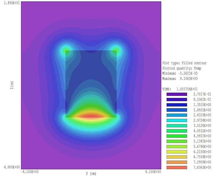
Figure 5. Temperature in the sample and surrounding air at 10 s, plot in the plane x = 0.0 cm.
The complete set of input files is available on request.
LINKS
